


This tutorial demonstrates how to use One-Click Optimization. It showcases how to run a multi-objective optimization and a single-objective optimization on Kursawe functions.
You must complete the Process Integration of Kursawe Functions tutorial before starting this one.
To set up and run the tutorial, perform the following steps:
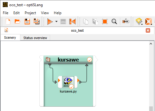
- Opening the Kursawe Process Integration Project
- Running the Multi-Objective Optimization Wizard
- Setting up the System for Multi-Objective Optimization
- Saving and Running the Multi-Objective Optimization
- Updating the Pareto 2D Postprocessing
- Multi-Objective Optimization Strategies
- Adding and Configuring Clusters
- Saving Postprocessing
- Running the Single-Objective Optimization Wizard
- Saving and Running the Single-Objective Optimization
- Viewing the Single-Objective Optimization Postprocessing
- Summary
Start optiSLang.
From the Start screen, click .
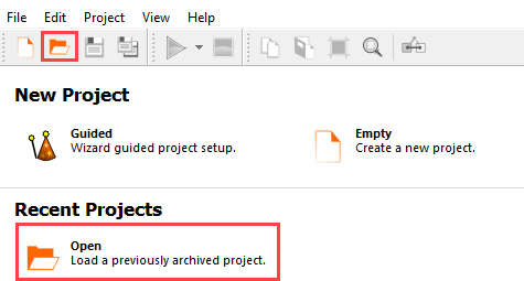
Browse to the location of the Kursawe process integration project you used in the previous tutorial and click .
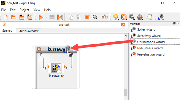
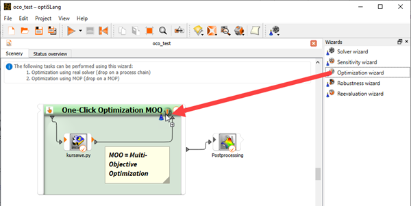
From the Wizards pane, drag the Optimization wizard to the head of the solver chain and let it drop.
Do not adjust the values in the Parametrize Inputs table.
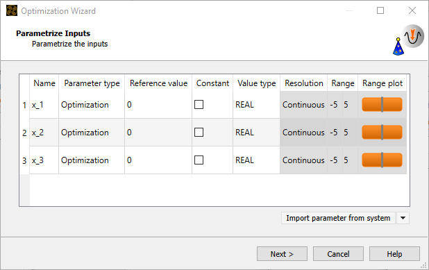
Click .
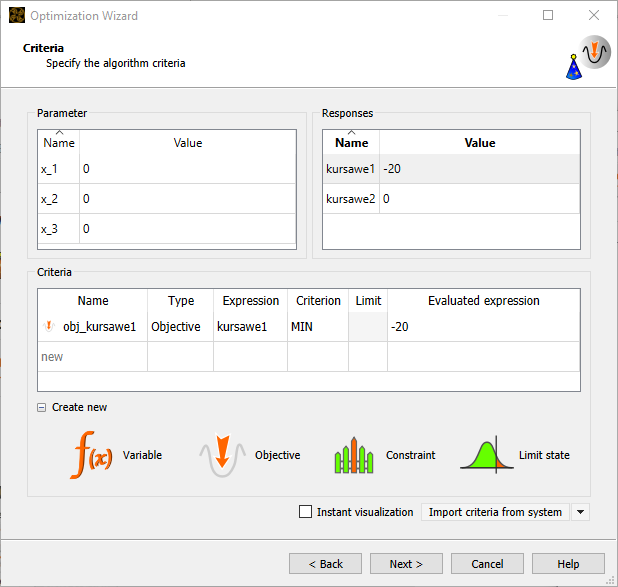
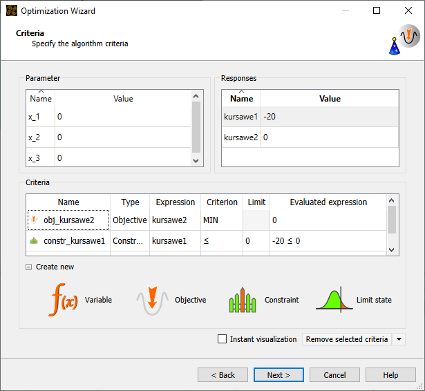
To define kursawe1 as a minimization objective, drag the row from the Responses table to the Objective Minimize icon and let it drop.
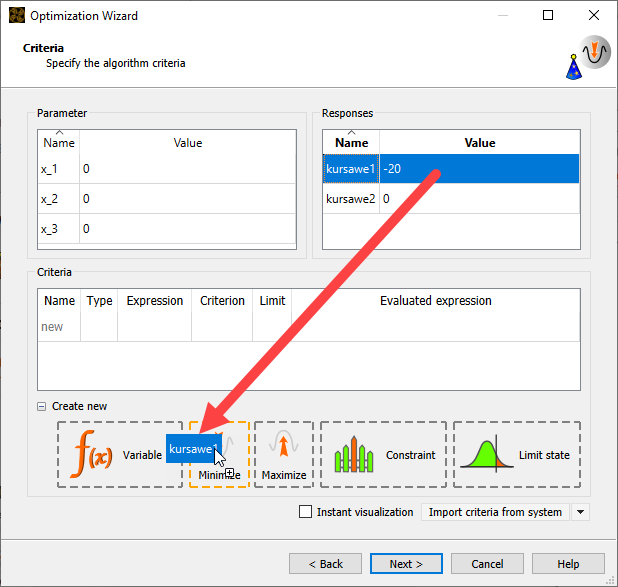
The objective is added to the Criteria table.
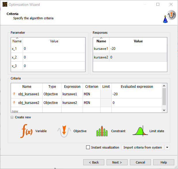
To define kursawe2 as a minimization objective, drag the row from the Responses table to the Objective Minimize icon and let it drop.
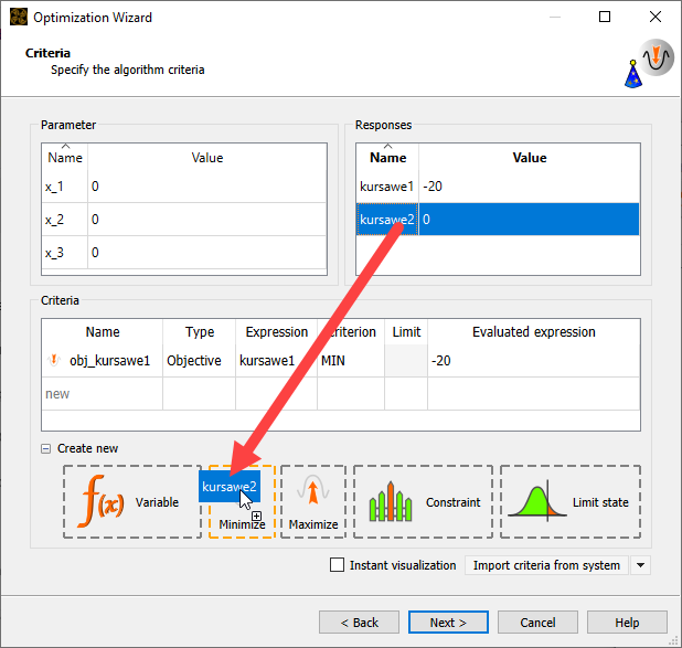
The objective is added to the Criteria table.
Click .
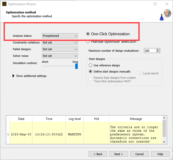
The One-Click Optimization is recommended and selected by default.
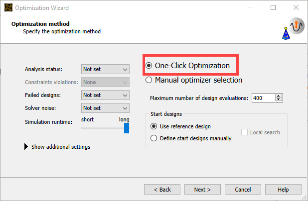
Since you did not conduct any Sensitivity analyses, set the Analysis status to . There is currently no information about Failed designs or Solver noise.
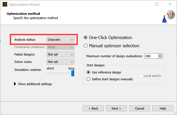
Leave the maximum number of design evaluations as-is, and click .
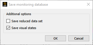
Do not change any of the additional options.
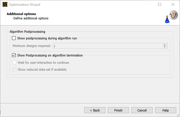
Click .
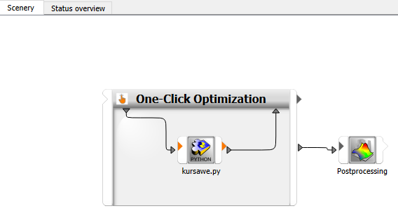
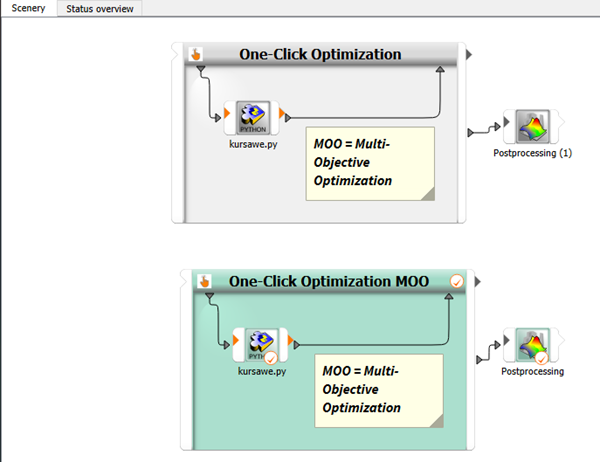
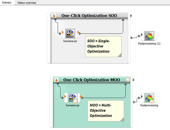
The One-Click Optimization system is created.
Right-click the One-Click Optimization system and select from the context menu.
Type
One-Click Optimization MOOand press Enter.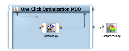
Right-click the One-Click Optimization MOO system and select > from the context menu.
In the note, enter
MOO = Multi-Objective
                        Optimization
.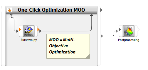
To save the project, click
 .
.Browse to the location to save the project and type a project name in the File name field.
Click .
To run the project, click
 .
.
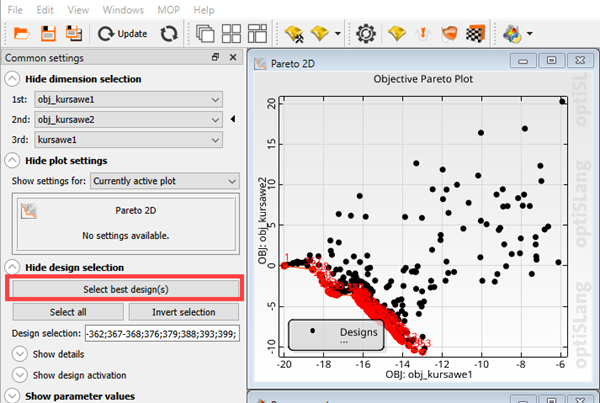
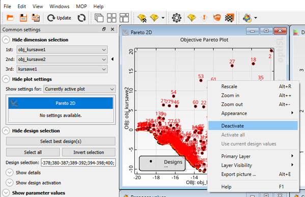
The Postprocessing window launches automatically after the project is run. It shows in the Pareto 2D plot the Pareto front and the conflicting objectives.
To select the best designs at the Pareto front, click .
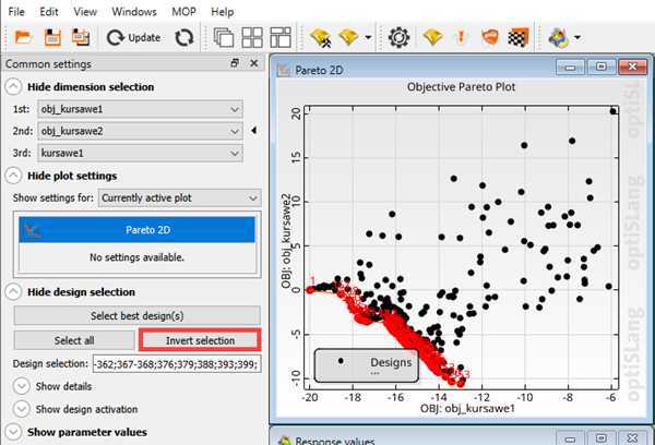
To investigate designs at the Pareto front only, click .
Right-click the Pareto 2D plot and select from the context menu.
A Posteriori Preference Articulation
Search before making decisions.
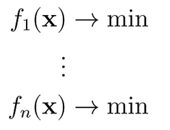
Multi-objective (Pareto) optimization
Find Pareto optimal solutions and choose the most suitable one.
Strategies to Continue
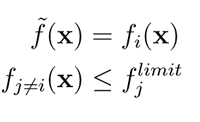
Strategy A:
Only the most important objective function is used as optimization goal
Other objectives as constraints
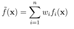
Strategy B:
One objective as sum of single criteria
Scale and weight single criteria
You continue with Strategy A.
From the Visuals pane, drag the Parallel coordinates plot from the Data mining folder into the window.
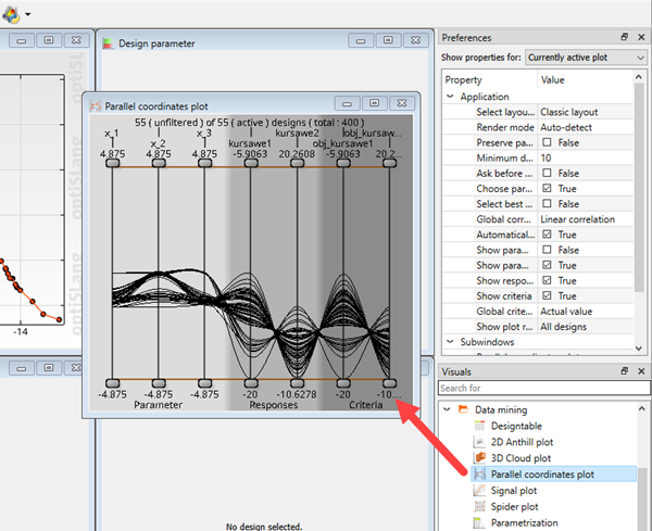
The Parallel coordinates plot is useful to understand a multidimensional space, set preferences and understand dependencies. Each line represents one design.
From the menu bar select > > .
In the Cluster Dialog, select and .
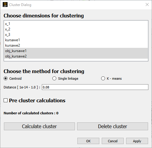
Select the K-means method for clustering
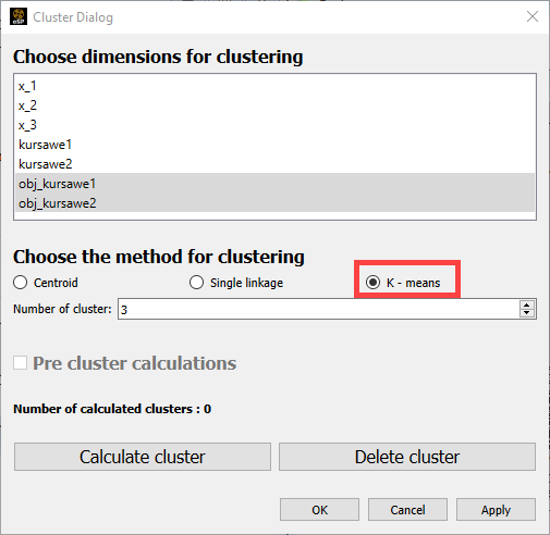
Click .
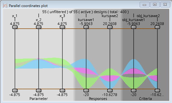
Click .
The conflict between the objectives is displayed in the Parallel coordinates plot.
To save the postprocessing, click
.Select .
Click .
To close the Postprocessing window, from the menu bar select > .
In the dialog box, click .
From the Wizards pane, drag the Optimization wizard onto the One-Click Optimization MOO system and let it drop.
Do not adjust the values in the Parametrize Inputs table.
Click .
To delete the existing objective for obj_kursawe1, right-click it and select Remove selected criteria from the context menu.
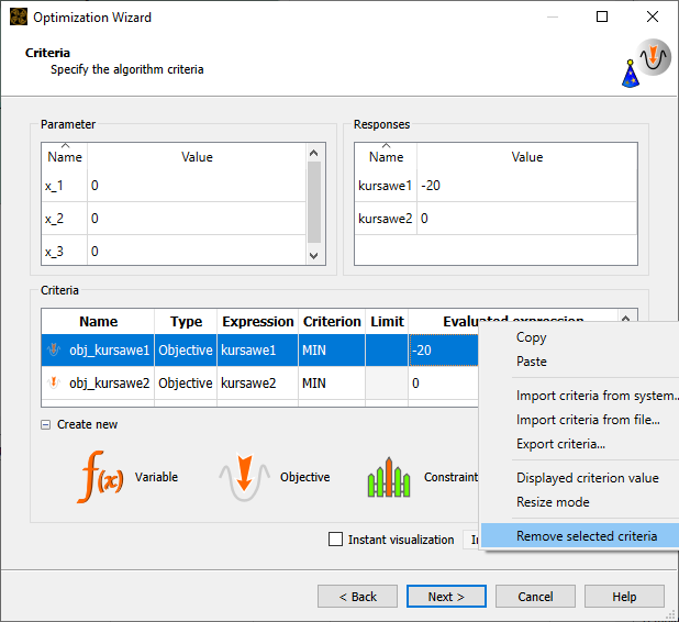
In the confirmation dialog box, click .
To define kursawe1 as a constraint, drag the row from the Responses table to the Constraint Less icon and let it drop.
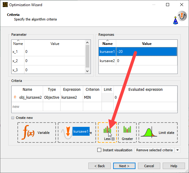
The constraint is added to the Criteria table.
In the Limit field for constr_kursawe1, enter
-14.5.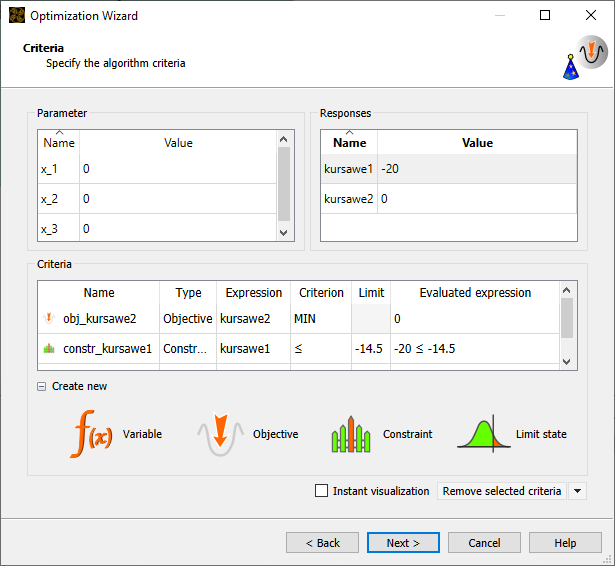
Click .
The One-Click Optimization is recommended and selected by default. The analysis status is automatically set.
Change the maximum number of design evaluations to
500.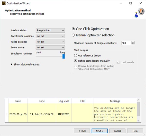
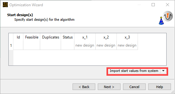
Keep Define start design manually.
Start designs cannot be automatically received from the One-Click Optimization MOO because you have changed the criteria.
Click .
Click .
We want to use the best design, which was design 327 from the Multi-Objective Optimization, to be our start design for the Single-Objective Optimization The design has the lowest value of obj_kusawe2 where obj_kusawe1 < -14.5 is still given.
In the Select system pane, click One-Click Optimization MOO.
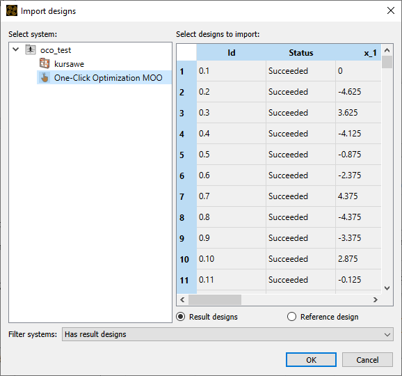
From the table, select line 327.
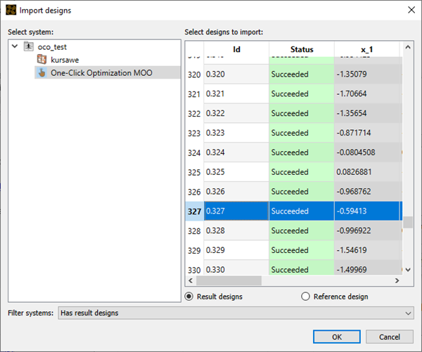
Click .
Click .
Do not change any of the additional options.
Click .
A new system is created.
To save the project, click
.To run the project, click
.
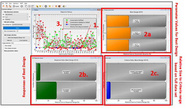
The Postprocessing window launches automatically after the project is run. The optimizer converges after 420 designs. The postprocessing displays the following information:
The best design, Design 310, has been automatically selected.
For this design, the following are shown:
Parameters
Responses
Criteria
The blue Convergence line in the History plot shows the improvement of the design during optimization.
Process Integration was conducted to automate the process.
With the One-Click Optimizer and without further configuration, the Pareto front is well captured.
The Multi-Objective Optimization showed the conflict of the optimization goals.
Define a strategy to find a Pareto optimal solution and choose the most suitable one.
Continue with a constrained, local Single-Objective Optimization.
Initial design :
Best Objective (Kursawe 2) : 0
Constraint (Kursawe 1) : -20.0 ≤ -14.5
Solver runs: 1.
Multi-objective optimization:
Objective (Kursawe 2) : -7.9
Objective 2 (Kursawe 1) : -14.5 ≤ -14.5
Solver runs: 400.
Single-objective optimization:
Best Objective (Kursawe 2) : -8.2
Constraint (Kursawe 1) : -14.5 ≤ -14.5
Solver runs: 420.