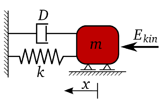
This tutorial allows you to complete an optimization of a single degree-of-freedom system excited with initial kinetic energy.

The equation of motion of free vibration is:

The un-damped and damped eigen-frequency is

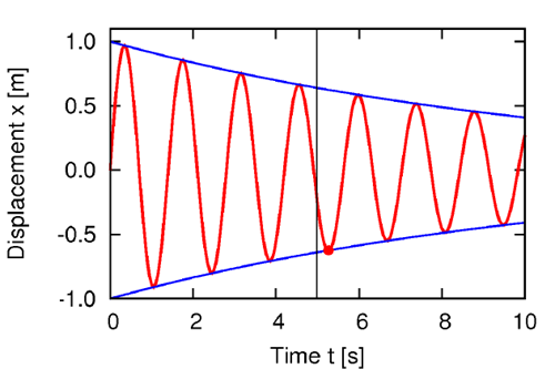
The time-dependent displacement function is:

The optimization goal is to minimize maximum amplitude after five seconds of free vibration.

The restricted damped eigen-frequency as the optimization constraint is:

The mass and stiffness as optimization variables, damping ratio and kinetic energy as the constant is:

This tutorial demonstrates how to do the following:
Generate a solver chain using text-based input and output
Define the input and output parameters
Perform a sensitivity analysis with respect to mass and stiffness using the global bounds

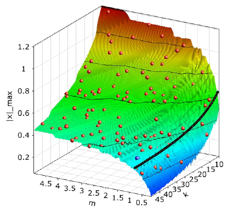
Perform a single objective and constrained optimization by minimizing the maximum amplitude
Perform an optimization using the Metamodel of Optimal Prognosis (MOP)
Perform an optimization using the Adaptive Metamodel of Optimal Prognosis (AMOP)
Before you start the tutorial, download the oscillator_optimization_calibration zip file from here , and extract it to your working directory.
To set up and run the tutorial, perform the following steps:
- Creating a New Project
- Starting the Solver Wizard
- Selecting the Input File
- Defining the Input Parameters
- Editing the Parameter Properties
- Selecting the Output File
- Defining the Response
- Defining the Optimization Criteria
- Importing the Solver Call Files
- Creating the Solver Chain Template
- Saving and Running the Project
- Completing the Sensitivity Wizard
- Running the Sensitivity Analysis
- Completing the Optimization Wizard using the MOP
- Running the MOP Optimization
- Adjusting the Optimization
- Completing the Optimization Wizard using the Adaptive MOP
- Configuring AMOP Settings
- Running the Project and Viewing AMOP Postprocessing
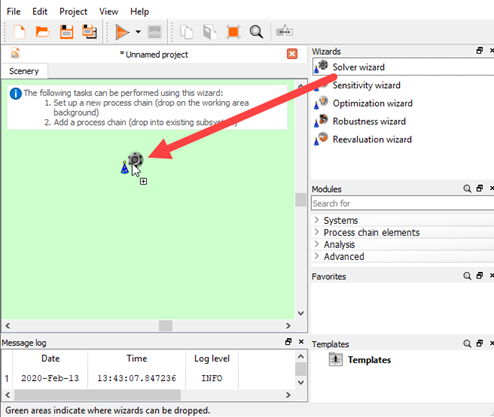
From the Wizards pane, drag the Solver wizard to the Scenery pane and let it drop.
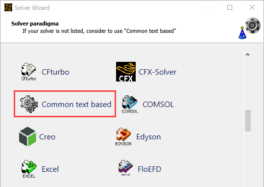
From the solver list, click .
In the Select input file dialog box, browse to the oscillator_optimization_calibration folder and select oscillator.s.
Click .
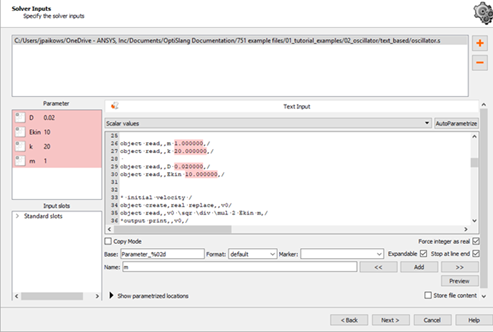
In the text editor, highlight lines 26-30
Click .
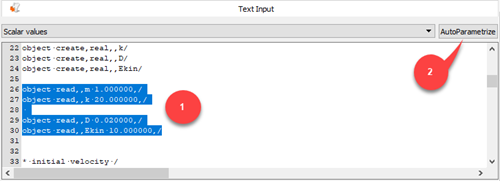
All possible values are marked.
Change the parameter name to
m.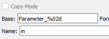
To register the parameter, click Add.
Repeat this procedure for parameters k, D, and Ekin.
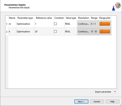
Click .
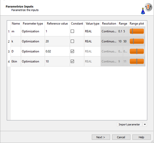
In row 1 (m), change the lower bound to
0.1and the upper bound to5.In row 2 (k), change the lower bound to
10and the upper bound to50.In rows 3 and 4 (D and Ekin), select the Constant check box.
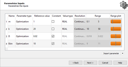
Click .
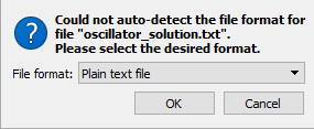
In the Choose a file to open dialog box, browse to the oscillator_optimization_calibration folder and select oscillator_solution.txt.
Click .
From the File format list, ensure is selected and click .
Highlight the text in line 1 (omega_damped).
Right-click the selection and select > from the context menu.
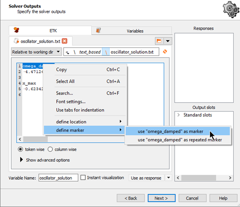
The response name is automatically taken from the marker.
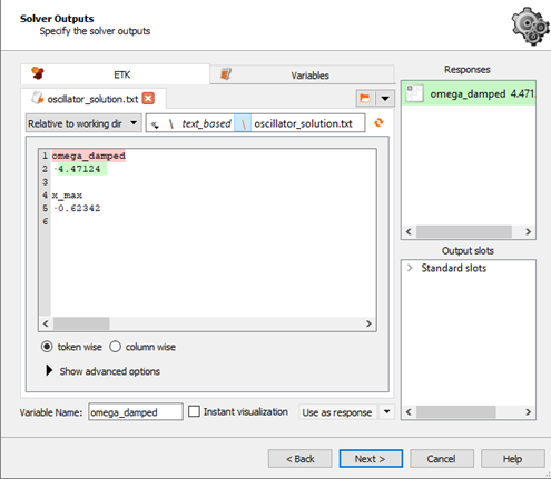
To register the value as a response, click .
The response is displayed in the Responses pane.
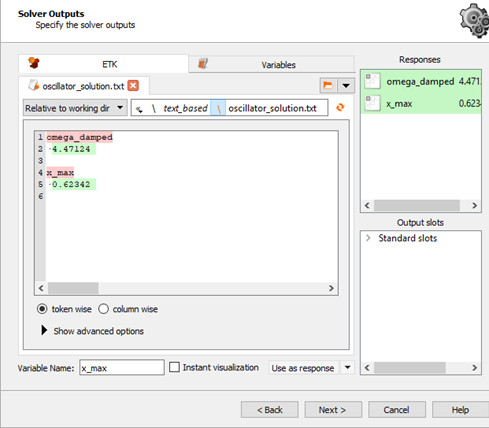
Repeat steps 2-4 for the x_max value.
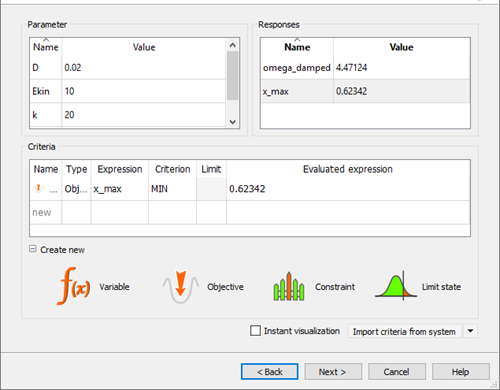
Click .
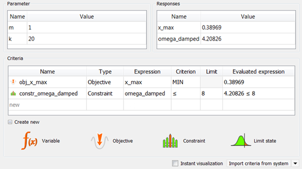
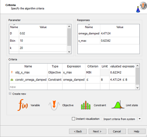
To define x_max as a minimization objective, drag the row from the Responses table to the Objective Minimize icon and let it drop.
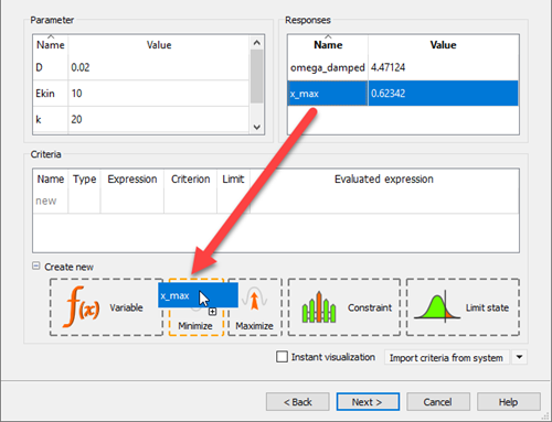
The new criterion is displayed in the Criteria table.
To define omega_damped as a constraint, drag the row from the Responses table to the Constraint Less icon and let it drop.
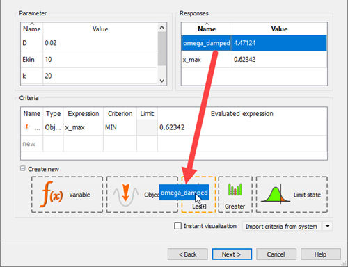
In the Limit field, enter
8.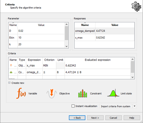
Click .
To the right of the Absolute path field, click the orange folder.
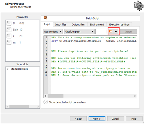
Browse to the oscillator_optimization_calibration folder and select oscillator.bat for Windows systems or oscillator.sh for Linux systems.
Click Open.
Click .
Select the Create a template from solver chain check box.
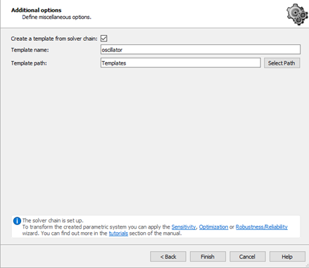
Click .
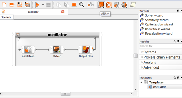
The template is displayed in the Templates pane and the system is displayed in the Scenery pane.
To save the project, click
 .
.Browse to the location to save the project and type a project name in the File name field.
Click .
To run the project, click
 .
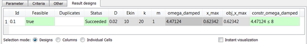
.To review the result, double-click the oscillator template and switch to the Result designs tab.
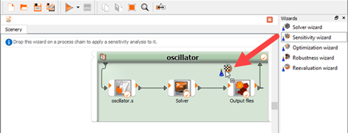
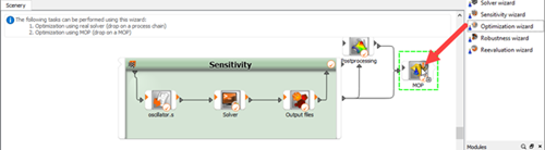
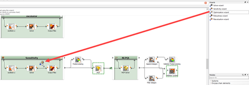
From the Wizards pane, drag the Sensitivity wizard to the head of the oscillator system and let it drop.
Do not adjust the values in the Parametrize Inputs table.
Click .
Do not adjust or add to the currently displayed values for parameters, responses, and criteria.
Click .
Select the Full factorial sampling method and leave the number of samples at 100.
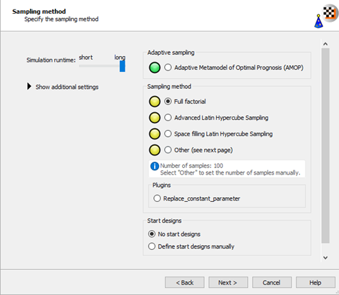
Click .
Do not adjust the current additional option settings.
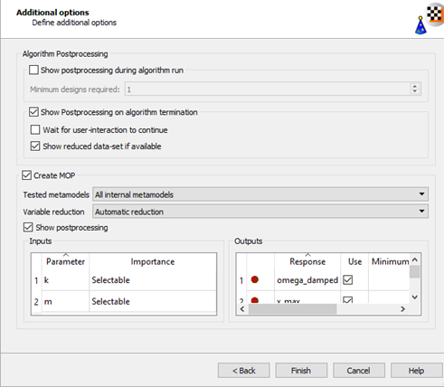
Click .
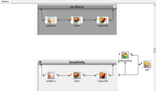
The Sensitivity system is displayed in the Scenery pane.
To save the project, click
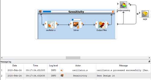
.To start the sensitivity analysis, click
.The bar on top of the sensitivity system displays the progress of the analysis. The message log displays the sequence of events.
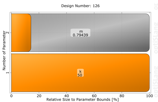
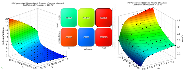
The results of the sensitivity analysis are displayed. You can observe:
The approximation quality is excellent for both responses
The influence of the inputs is contrariwise
Drag the Optimization wizard onto the MOP node and let it drop.
Do not adjust the values in the Parametrize Inputs table.
Click .
Do not adjust or add to the currently displayed values for parameters, responses, and criteria.
Click .
Click .
Do not adjust the current optimization method settings.
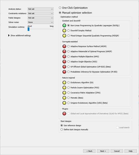
The gradient based NLPQL is recommended.
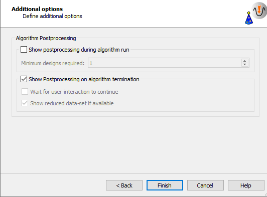
Leave the additional optional settings at the default and click .
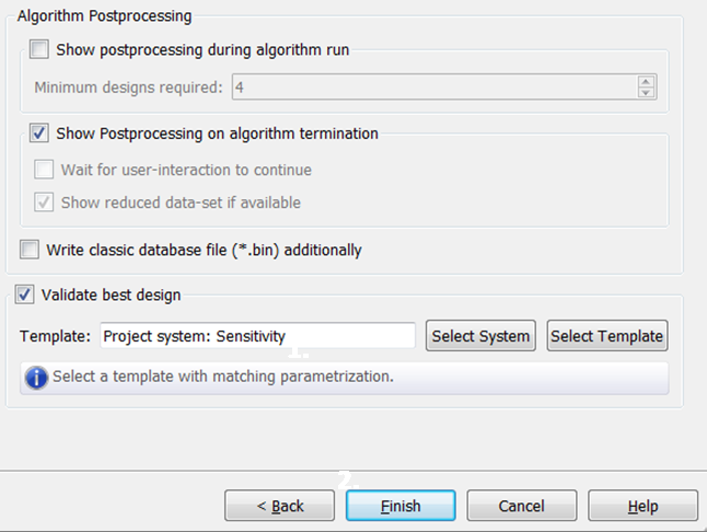
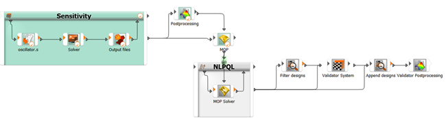
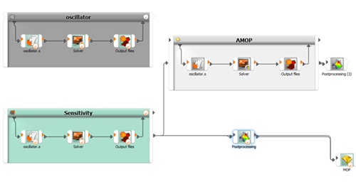
The scenery is extended with the optimization and validation workflow.
To save the project, click
.To run the project, click
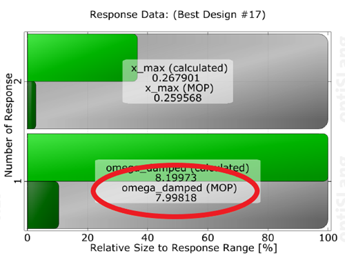
.The optimizer converges within a few iterations. The response, objective, and constraints of the best design are verified. Due to local approximation errors, the constraints of the best design may be violated in the validation solver run. Validation of the best design is very important for the optimization on the MOP .
If the validation is not satisfactory (for example, a large discrepancy or a violated constraint), use the following alternative strategies:
Change the constraint to provide a safety margin.
Append a local re-optimization with a direct solver call, using the best design on MOP as the starting design. The best design can be passed automatically to the new optimization system. However, we do not recommend using an infeasible start design.
Improve the metamodel locally by adding a validated best design to the sensitivity design of experiments and build a new metamodel, then repeat the optimization.
Drag the Optimization wizard onto the Sensitivity node and let it drop.
Do not adjust the values in the Parametrize Inputs table.
Click .
Do not adjust or add to the currently displayed values for parameters, responses, and criteria.
Click .
Click .
Do not adjust the current optimization method settings.
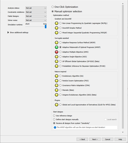
The Adaptive Metamodel of Optimal Prognosis (AMOP) is recommended. All previous designs are considered as start designs.
Click .
Leave the additional optional settings at the default and click .
The AMOP system is connected to the sensitivity system.
Double-click the AMOP system to open the settings.
On the Adaption tab, select the Show advanced settings check box.
In the Maximum number of samples field, enter
45.Adjust the refinement sliders so the first two are at 0% and the Importance of optimization criteria slider is at 100%
In the Maximum iterations field, enter
10.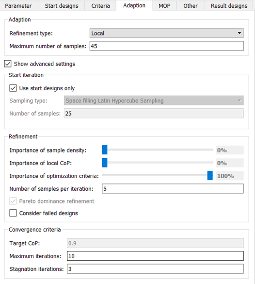
To save and close the settings, click .
To save the project, click
.To run the project, click
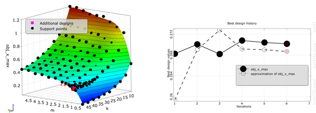
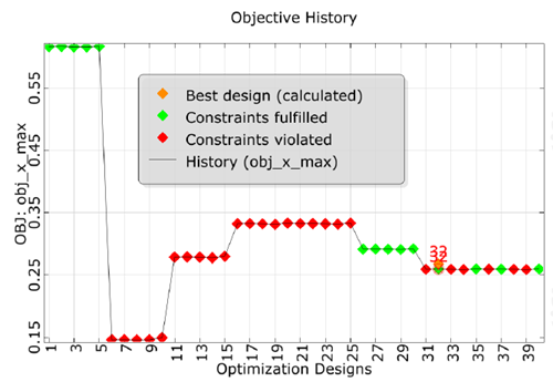
.The AMOP postprocessing is displayed. You can observe:
The AMOP with criteria refinement converges in a few iteration steps to the global optimum
Validation of best design is performed in every iteration
The history plot compares best design approximation and validation