


This tutorial allows you to complete an optimization of the Kursawe Functions.
This tutorial demonstrates how to do the following:
Use the parameter and response definitions from the sensitivity analysis
Perform a single, objective, and constrained optimization by minimizing Kursawe2
Kursawe2 → min
Kursawe1 < -14.5
Perform optimization on the Metamodel of Optimal Prognosis (MOP) from the sensitivity analysis
Perform direct optimization in the full parameter space using the Adaptive Metamodel of Optimal Prognosis (AMOP)
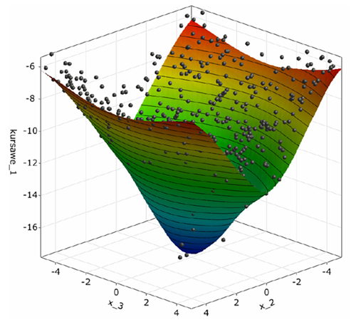
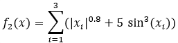
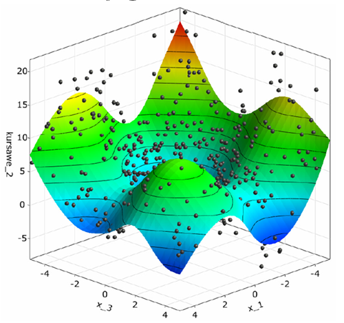
The Kursawe Functions
Objective function one has one dominant global optimum. Objective function two has four local optima.

You must complete the Sensitivity of Kursawe Functions tutorial before starting this one.
To set up and run the tutorial, perform the following steps:
Start optiSLang.
From the Start screen, click .

Browse to the location of the Kursawe process integration project you used in the previous tutorial and click .
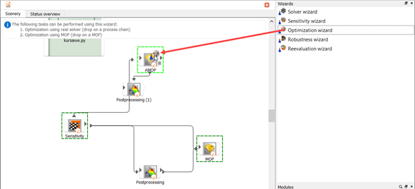
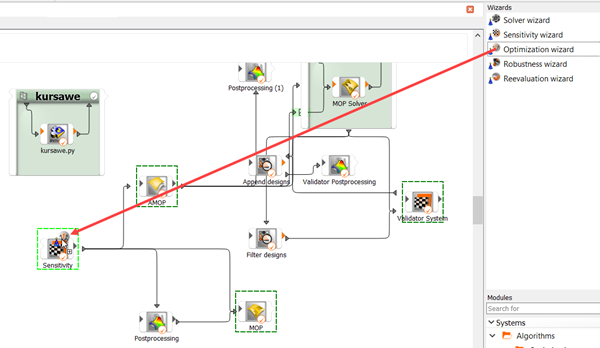
Right-click the Sensitivity system and select from the context menu.
Repeat step 4 for the AMOP system.
From the Wizards pane, drag the Optimization to the AMOP node and let it drop.
Do not adjust the values in the Parametrize Inputs table.
Click .
Do not adjust the values in the Parameter, Responses, or Criteria tables.
Click .
Click .
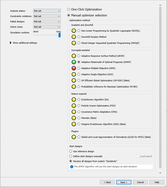
Do not adjust the current optimization method settings.
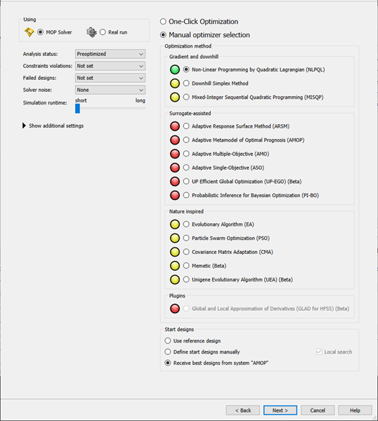
The gradient based NLPQL is recommended. Start designs are automatically received from the AMOP system.
Click .
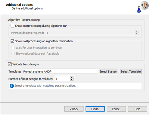
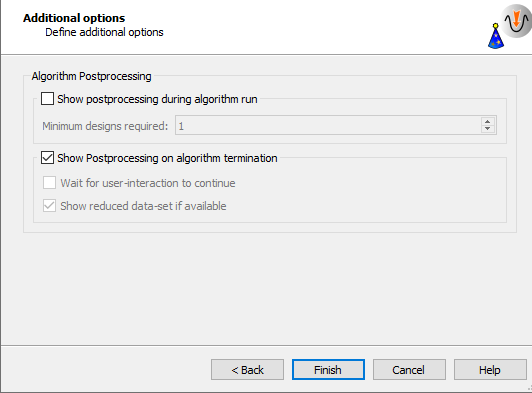
Leave the additional optional settings at the default and click .
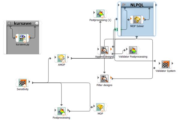
The optimization and validation flow is added to the Scenery pane.
To save the project, click
 .
.To run the project, click
 .
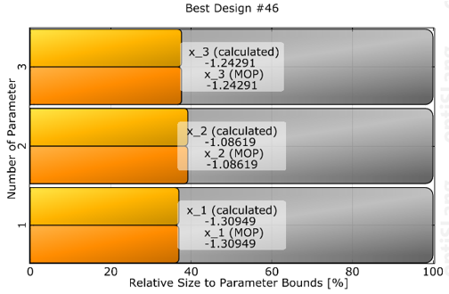
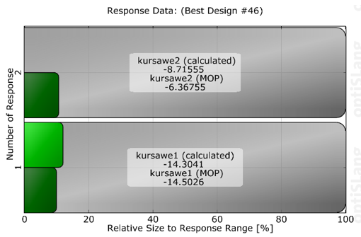
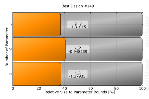
.The optimizer should converge in a few iteration steps. The response and objective of the best design are verified with the solver. Due to local approximation errors, the estimated response value may differ from the solver result. Validation of the best design is necessary. The validation shows that the constraint is violated.
Local Optimization
If the validation of the optimum is not satisfactory (for example, a large discrepancy or a violated constraint), use the following continuation strategies:
Change the constraint in order to provide a safety margin.
Append a local re-optimization with a direct solver call, using the best design on MOP as the starting design. The best design can be automatically passed to the new optimization system. However, using an infeasible start design is not recommended.
Improve the metamodel locally. Add the validated best design to the Sensitivity DoE and build a new metamodel, then repeat the optimization.
From the Wizards pane, drag the Optimization to the Sensitivity node and let it drop.
Do not adjust the values in the Parametrize Inputs table.
Click .
Do not adjust the values in the Parameter, Responses, or Criteria tables.
Click .
Click .
Do not adjust the current optimization method settings.
The Adaptive Metamodel of Optimal Prognosis (AMOP) is recommended. All previous designs are considered as start designs.
Click .
Leave the additional optional settings at the default and click .
The AMOP system is connected to the previous sensitivity system. The best design of the previous optimization is imported automatically.
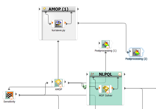
Right-click the AMOP (1) system and select from the context menu.
Change the name to
AMOP_localand press Enter.
Double-click the AMOP_local system to open the settings.
On the Adaption tab, select the Show advanced settings check box.
Adjust the refinement sliders so the first two are at 0% and the Importance of optimization criteria slider is at 100%
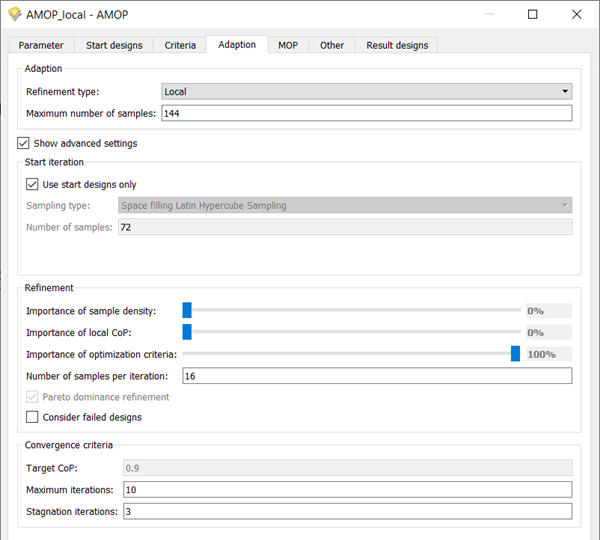
To save and close the settings, click .
To save the project, click
.To run the project, click
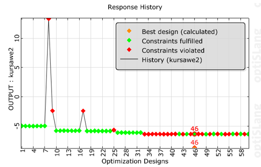
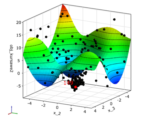
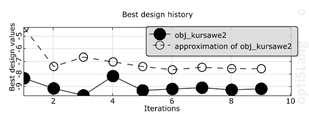
.The AMOP postprocessing is displayed. You can observe:
The AMOP with criteria refinement converges in a few iteration steps to the global optimum
Validation of best design is performed in every iteration
The history plot compares best design approximation and validation
The tutorial showed that:
Sensitivity analysis indicated all design variables as important
Optimization on the MOP lead to good optimal design
Optimization in the full parameter space could be obtained efficiently by the AMOP
| Method | Best Objective (kursawe2) | Constraint (kursawe1) | Solver Runs |
|---|---|---|---|
| Initial design | 0 | -20.0 ≤ -14.5 | 1 |
| Sensitivity analysis | -4.9 | -15.4 ≤ -14.4 | 100 (300 with AMOP) |
| NLPQL on MOP | -8.7 | -14.3 > -14.5 | 1 |
| AMOP with local refinement | -8.2 | -14.5 ≤ -14.5 | 100 + 144 |