


In this tutorial, you will perform a MAC analysis to determine the degree of consistency between mode shapes for an Ansys Mechanical modal analysis and experimental results.
| Analysis Type | Modal Assurance Criterion (MAC) |
| Features Demonstrated | NVH Toolkit Add-on, NVH toolkit system, MAC calculator, node matching algorithm and panes explanation, node mapping algorithm, cycling optimization option,complex to real projection |
| Licenses Required | Ansys Mechanical Premium/Enterprise/Enterprise PrepPost |
| Help Resources | NVH Toolkit Add-on |
| Tutorial Files | NVHMacCalculator.zip |
This tutorial guides you through the following topics:
The MAC Calculator introduces a result in the project tree that calculates the Modal Assurance Criterion (MAC) between Ansys Mechanical modal analysis results (rst) and experimental results (unv) or between two different rst results. In this tutorial, you will perform a MAC analysis to determine the degree of consistency between mode shapes for an rst vs unv case.
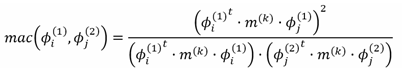
The MAC between two real solutions is computed using the equation:
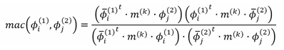
The MAC between two complex solutions is computed using the equation:
Refer to the MAC Calculation Method documentation for further information.
Data files for this tutorial can be found here on the Ansys customer site.
The zip folder contains the following files:
MAC_Model_Addon_Unsolved.wbpz - this is the input model that you will set up in the steps below. Copy this file to a working folder and complete the worked example.
file_tutorial.unv - a file in unv format used in the MAC calculation.
MAC_Model_Addon_Completed.wbpz - this is an example of the completed model once all the steps have been followed.
Make the NVH Toolkit Add-on available in Mechanical
Start Workbench, and select > .
Browse to the working folder and select MAC_Model_Addon_Unsolved.wbpz.
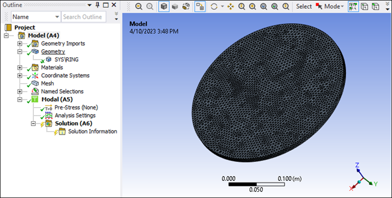
This Workbench project contains the Modal analysis system.
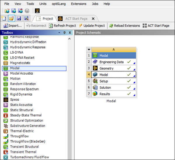
Double click the Model cell to open Mechanical.
To make the NVH Toolkit capabilities available, click the icon in the ribbon.
The icon is highlighted in blue, indicating that the add-on is loaded.
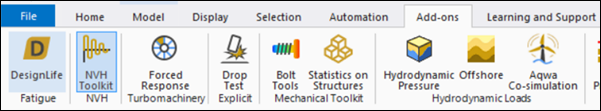
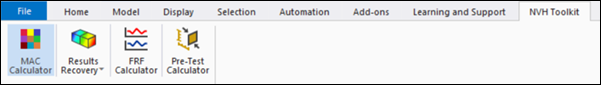
Once the add-on is loaded, the Ansys NVH Toolkit ribbon is visible, exposing all the NVH capabilities.
Verify geometric model
The geometry consists of a solid body, as shown in the figure below.
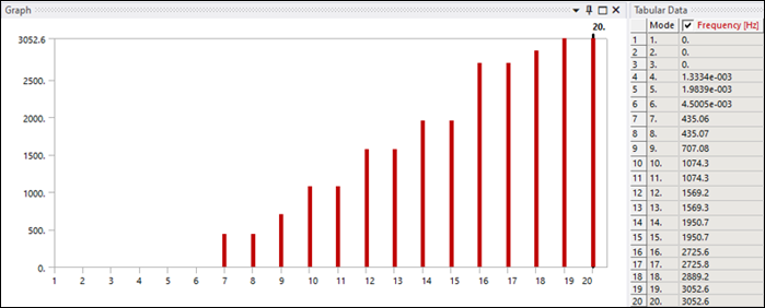
Solve modal analysis
To verify that the object is fully defined, right-click the Model or Solution and solve the analysis.
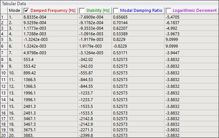
Verify the natural frequencies or eigenvalues (see below).
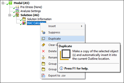
Right-click the Modal solution and insert a result. Confirm that it is in an undefined state with default Details as shown below.
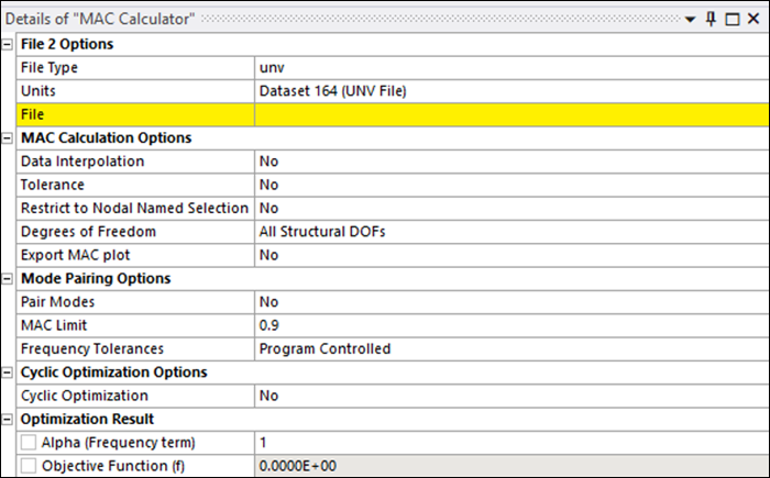
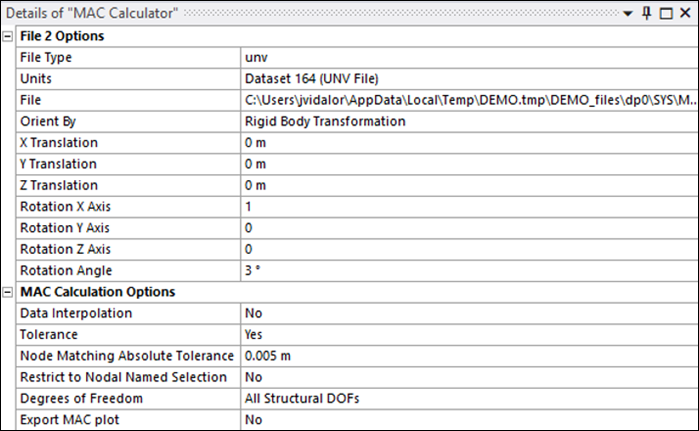
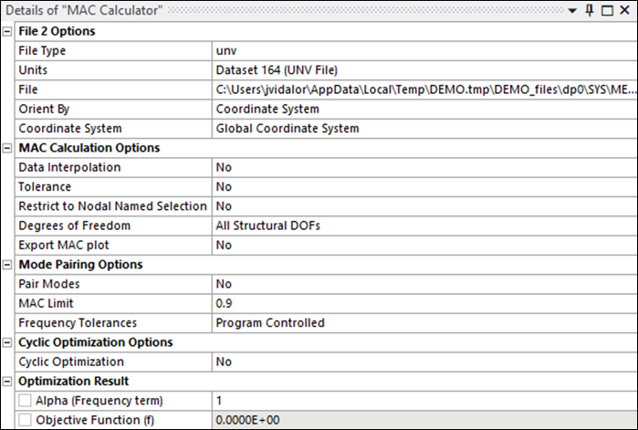
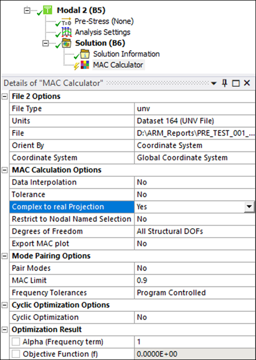
Set the Details for the MAC Calculator object as shown below.
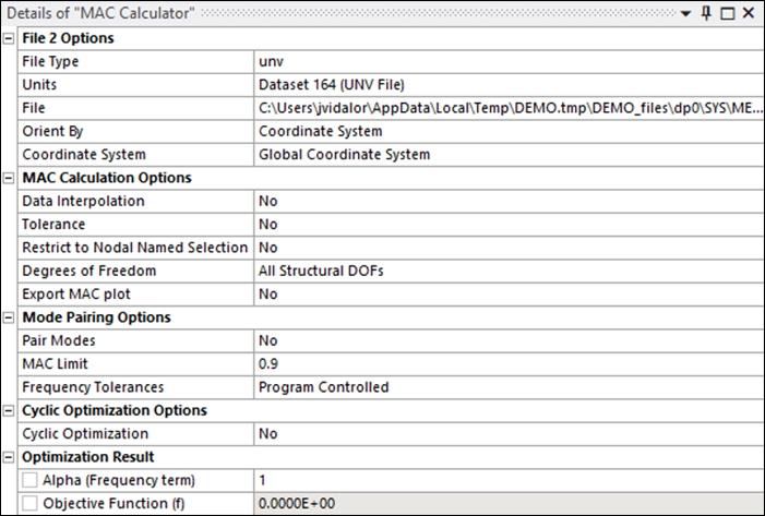
File 2 Options > File Type currently supports rst or unv files. For this case, select the unv file for this tutorial.
File 2 Options > Orient By property has three options which will help you in unv positioning. Refer to the MAC Calculation Options documentation to for information on additional functionality.
Note that a UNV Node Worksheet has been generated. It is only available after loading a unv file.
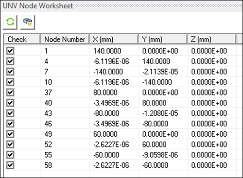
A check mark for a listed node indicates that the node will be employed in subsequent MAC calculations.
Manually editing the coordinates should be done after aligning the rst and unv models through the properties listed under File 2 Options in the MAC Calculator Details panel. If the nodes are edited and then any option (Coordinate System/RB Transformation/3 Node Alignment) is changed, the node location is reset.
Refer to UNV Node Worksheet for more information about the functionality of this Worksheet.
MAC Calculation Options will be described in the course of this tutorial. Data Interpolation allows you to choose if you want to use a node matching algorithm (Step 6 of this tutorial) or node mapping algorithm (Step 7 of this tutorial). The Complex to Real Projection property will be explored in Step 9 of this tutorial (it is only available if just one of the 2 files has complex modes). You can restrict the analysis to a Nodal Named Selection from File 1, or to certain Degrees of Freedom, using the corresponding property.
The MAC plot can also be exported in .png format.
Mode Pairing Options allow you to enable and customize the Automatic Mode Pairing Algorithm. You can select the MAC Limit for this algorithm, as well as Frequency Tolerances (, and ).
Cyclic Optimization Options are covered in Step 9. These options are only supported for unv files. These options are used to enable a specific workflow useful for models that exhibit cyclic (cylindrical) symmetry. In these cases, both rst and unv models can produce bending modes at random azimuthal angles, and these options are enabled to provide the best possible correlation between them. This is performed by rotating the unv model according to the options below and providing the best match from all the possible configurations.
Optimization Result options provide an indicator of the quality of the correlation between File 1 and File 2 modes. It is a minimum objective function, which means that two perfectly well-correlated models yield an optimum value of 0. Refer to Objective Function Formulation in the documentation for further details.
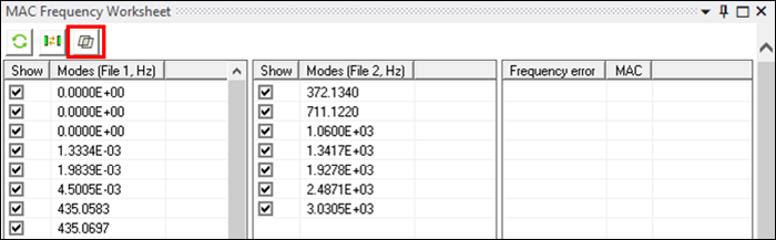
The button is available in the MAC Frequency Worksheet under the following conditions: MAC Calculation Options > Data Interpolation is set to , data from File 1 and File 2 is available, but the MAC Calculator has not been generated.
This option allows you to see a preview of the matching nodes used for your selected options. If Tolerance is set to , it will match every node from the first file to a node from the second file, with a nearest match node algorithm.
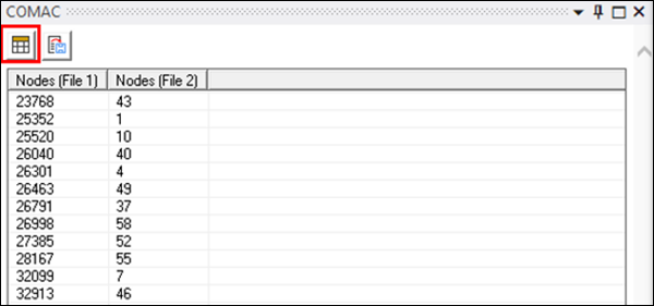
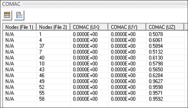
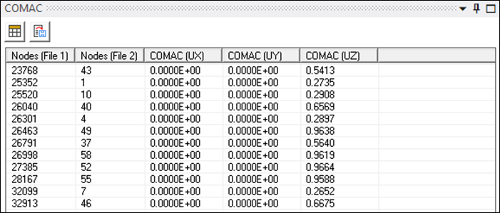
Click this button and observe that COMAC table is shown, with the following results:
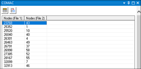
If you select a row, you will see in the model the nodes from both files used for MAC calculation.
Update the details for the MAC Calculator object as shown below (notice that you set a value for the Tolerance). Observe that COMAC table is cleaned.
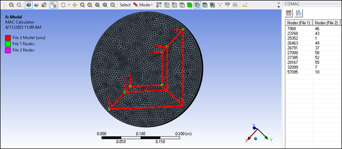
Click the button again and observe that in this case, only 10 nodes are displayed in the COMAC table, as those are the only node pairs that comply with the Tolerance property.
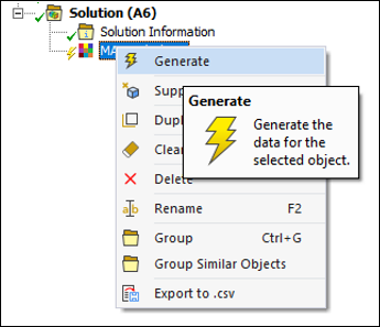
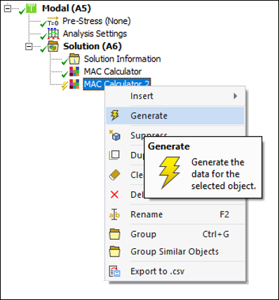
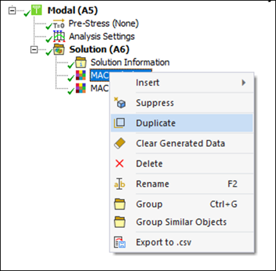
Reset the Details properties as in Step 5b of this tutorial and generate the MAC Calculator by right-clicking the MAC tree object and selecting (without clicking the button).
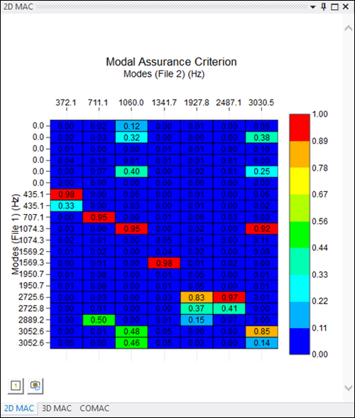
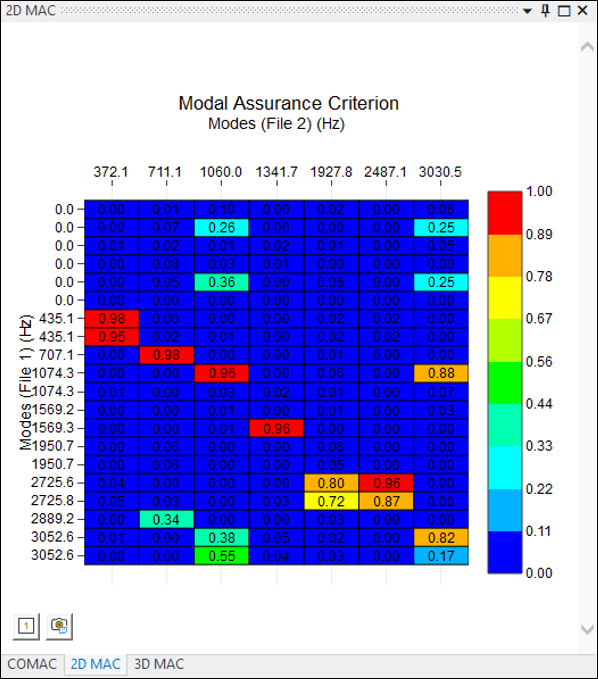
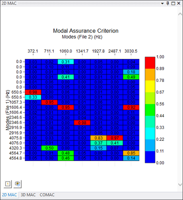
Go to the 2D MAC table and check the results. These results are calculated with the matched nodes, using the MAC real-to-real formulation. The File 1 modes are displayed in rows and the File 2 modes in columns, with the items of the table showing the MAC values of each pair of modes.
Hover in the table to inspect the individual values. Command buttons above the table enable you to , and the view of the table.
The 2D MAC table pane has two buttons:
Click the first button to the MAC values inside each item in the table.
Click the second button to the MAC table to png format in a selected folder. This can also done by selecting MAC Calculation Options > Export MAC plot (in this case it will be stored in your MAC folder).
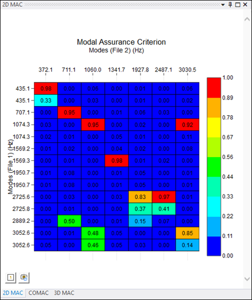
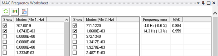
If the modes in the MAC Frequency Worksheet are checked/unchecked or moved upwards/downwards, the 2D MAC table is automatically refreshed. Uncheck the following modes in the MAC Frequency Worksheet:
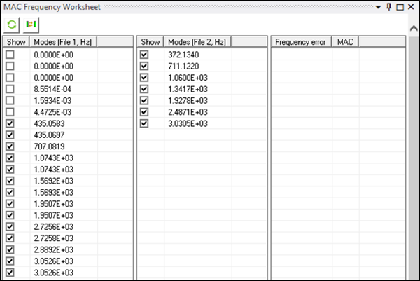
And observe that the 2D MAC table is dynamically updated:
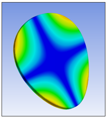
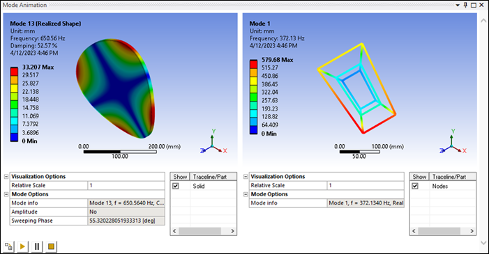
Click in the first item of 2D MAC table. This will display the Mode Animation view for that pair of modes (see below). You can graphically observe the animated mode shape. For this case, add a relative scale of
-1in the second file, to assist with visualization. Observe that the behaviour is practically the same for both files. This explains why this MAC value is0.981.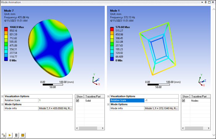
Click the 1st column - 3rd row item and observe that those mode shapes are completely different. This explains why you get a MAC value of
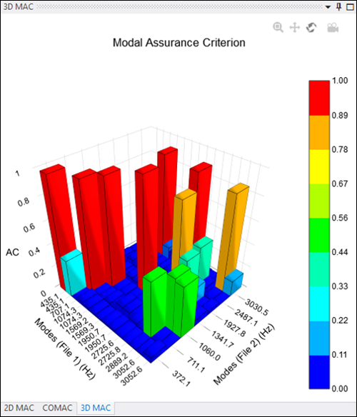
0.0. For further information, refer to Mode Animation View in the NVH documentation.The 3D MAC table is docked with 2D MAC table. Switch to this table and observe that the MAC value for each pair of modes is represented in a bar, defined by its height and color. The modes are displayed in the X and Y directions.
Hover in the table to inspect the individual values. Command buttons above the table enable you to switch between the , and mode, and to the camera.
If the modes in the MAC Frequency Worksheet are checked/unchecked or moved upwards/downwards, the 3D MAC table is automatically refreshed. In addition, when the or buttons are clicked in the MAC Frequency Worksheet, the 3D MAC table is automatically refreshed.
Go to the COMAC table and click the Compute COMAC button. Coordinate Modal Assurance Criterion (COMAC) is an extension to the MAC calculation that identifies the degrees of freedom that are the source of low correlation between the models. Refer to the Coordinate Modal Assurance Criterion Calculation section in the NVH documentation for further details.
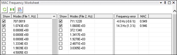
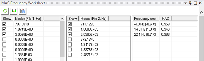
An error will be displayed, as you first need to pair modes. Go to the MAC Frequency Worksheet and click the button. Check that you get the following result:
Go back to COMAC table and click the button again. Check that you get these results:
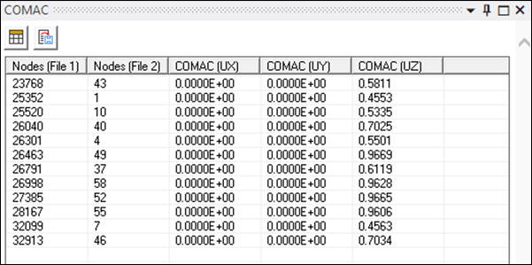
For this case COMAC values for UX and UY have a low degree of correlation. However, they do not have a major impact on the MAC value, as this is not the predominant DOF. Peripheral nodes, however, have a lower COMAC value than central nodes. If you look at the first paired mode, all the nodes have a similar behaviour. However, for the second paired mode, central nodes are the only ones showing the same behaviour for both files. This explains the difference in COMAC values. You can export COMAC data (any time) as well as MAC Frequency Worksheet data (after mode pairing).
Right-click the MAC Calculator tree object and select the option:
Notice that the button and Tolerance are no longer available.
Set Data Interpolation to and click the button. Notice that the button and Tolerance are no longer available. this new MAC analysis.
Check that you get the following results:
If you compare these values with those obtained with the Matching Node Algorithm, you will notice they are similar. The node-mapping algorithm interpolates results based on proximity.
For a non-refined mesh case and with localized mode shape effects, a greater difference will be observed (the node-matching algorithm can lead to distant nodes being matched). The advantage of node mapping is that you do not only consider one node (which may or may not be the one you are looking for), but you consider all the nodes from the first file. Based on their proximity to the second file, their equivalent contribution is considered.
For this refined, homogenous mesh with non-localized mode shape effects, results are similar.
Pair the modes and check that you get the following results:
Go to COMAC table and click the button. Check that you get the following results:
Results from the Mapping Node and Matching Node Algorithms are similar again for the same reason previously explained for MAC values. An
N/Avalue is observed in nodes from File 1, as the Mapping Nodes algorithm calculates the node2-equivalent result from the contribution of all the nodes in File 1, based on their proximity.The rest of the functionality is the same as for the Node Matching Algorithm.
Right-click the first MAC Calculator tree object and select the option.
Set Cyclic Optimization to and click the button. Notice that a Cylindrical Coordinate System is selected by default, as well as the Optimize By and Number Of Sectors options. this new MAC analysis.

Check that you get the following results:

Compare this with the results obtained with the Node Matching Algorithm in Step 6 of this tutorial. Note that the Cyclic Optimization values are higher, as they provide the best possible correlation between the rst and unv files after rotating the unv file.
Change the Number Of Sectors value to
36and regenerate the analysis. Observe that you get the following results: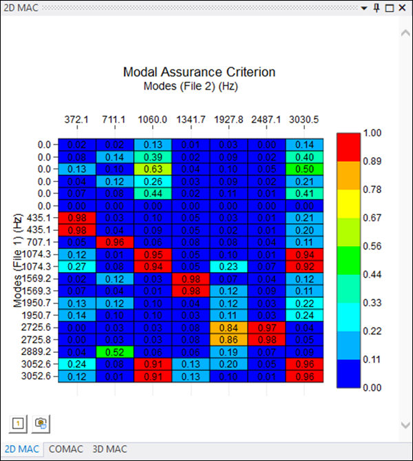
Although the lower MAC value results are different, higher MAC values present a low variation.
and check that you get the following results:
Note that you get 3 paired modes, instead of the 2 paired modes obtained with the Node Matching Algorithm.
Check that you get the following results:
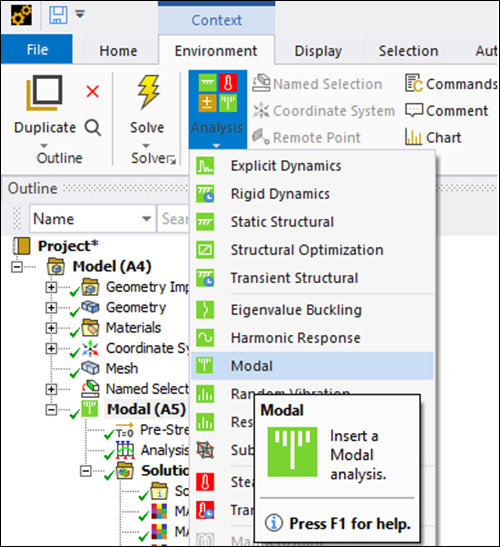
Click the Modal (A5) tree object and select Environment > Analysis > Modal.
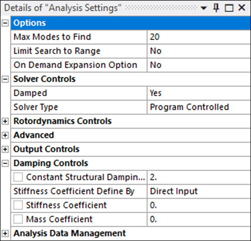
Set the following options:
Check that you get the following results:
Insert a new MAC Calculator analysis and set the following options. This is the same as for the Node Matching Algorithm, but with the Complex to Real Projection option enabled. This option is only available if one of the two files has complex modes and the other one has real modes. With this option, complex modes will be converted to real modes as explained in Complex to Real Projection Methodology in the NVH documentation.
this new analysis and check that you obtain the following results:
Compare these results with those obtained for the Node Matching Algorithm. Note that results are almost the same. To understand this, go to the MAC Frequency Worksheet and check that you get the following results for Modal Phase Collinearity (MPC). This is a parameter used to quantify the complexity of a mode. The lower the value, the more complex the mode is.
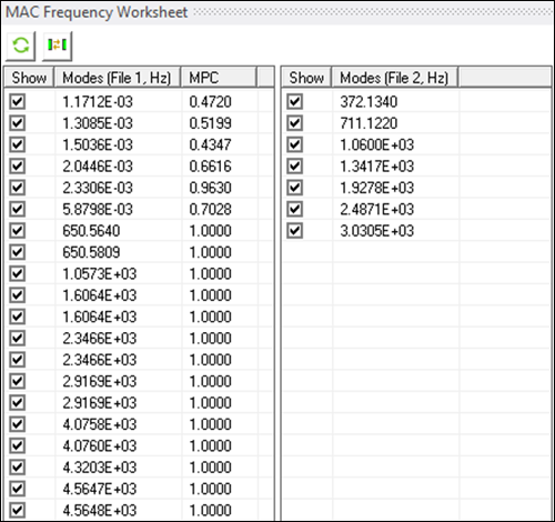
Note that MAC values have changed for modes with MPC lower than 1.
Check the results for Mode Animation from the 1st column, 7th row:
Note that modes from the first complex mode file show the sweeping phase used in the projection (read-only option in this case).
You have completed the Modal Assurance Criterion analysis and accomplished the overall objective for this tutorial.
Congratulations! You have completed the tutorial.