


In this tutorial, you will perform a frequency response analysis to determine the steady state vibration for a range of frequencies on a given structure.
| Analysis Type | Frequent Response Functions |
| Features Demonstrated | NVH Toolkit Add-on, NVH toolkit system, FRF calculator, FRF plots, FRF data |
| Licenses Required | Ansys Mechanical Premium/Enterprise/Enterprise PrepPost |
| Help Resources | NVH Toolkit Add-on |
| Tutorial Files | NVHFRF.zip |
This tutorial guides you through the following topics:
Frequency Response Functions are used to calculate the steady-state response at a particular point (degree-of-freedom) for a particular force input at a point (the same as the response point or another point). The FRF Calculator within the NVH toolkit introduces a result in the project tree that calculates the Frequency Response Function (FRF) for a given set of input and output degrees of freedom (DOFs). The method employs the residue formulation to estimate the FRF between two given degrees of freedom (DOFs) using modal parameters:

where the following notation is used:
 - FRF between the i-th and
j-th DOFs, where DOF i is the output and DOF
j is the input.
- FRF between the i-th and
j-th DOFs, where DOF i is the output and DOF
j is the input. - Number of modes considered in the FRF calculation.
 - r-th vibration mode, with
  its real part and
  its imaginary part:
Refer to the Add FRF Calculator documentation for further information.
In this tutorial, you will perform a frequency response analysis to determine the steady state vibration for a range of frequencies on a given structure.
Data files for this tutorial can be found here on the Ansys customer site.
The zip folder contains the following files:
FRF_Model_Addon.mechdat - this is the input model that you will set up in the steps below. Copy this file to a working folder and complete the worked example.
FRF_Model_Addon_Completed.wbpz - this is an example of the completed model once all the steps have been followed.
FRF Tutorial Worksheet.xlsx – refer to Step 6f of this tutorial for more information.
Start Workbench, and select > .
Browse to the working folder and select MFRF_Model_Addon.mechdat.
This Workbench project contains the Modal analysis system.
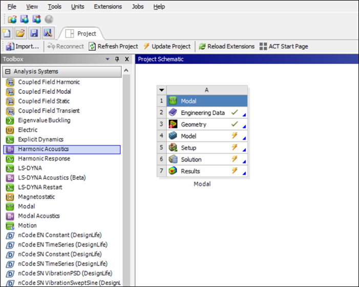
Double click the Model cell to open Mechanical.
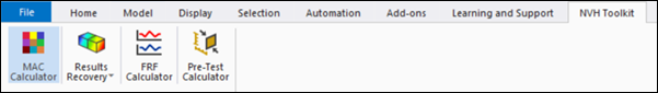
To make the NVH Toolkit capabilities available, click the icon in the ribbon.
The icon is highlighted in blue, indicating that the add-on is loaded.
Once the add-on is loaded, the Ansys NVH Toolkit ribbon is visible, exposing all the NVH capabilities.
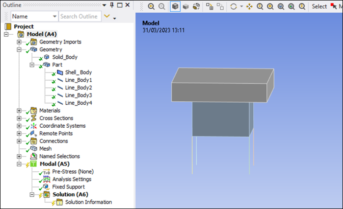
Verify geometric model
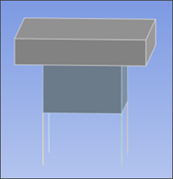
The geometry consists of a solid body, a shell body and four line bodies as shown in the figure below.
Solve modal analysis
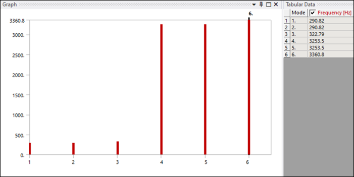
To verify that all the tree objects are fully defined, right-click the Model or Solution and solve the analysis.
Verify the natural frequencies or eigenvalues (see below).
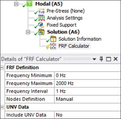
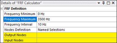
Right-click the Modal solution and insert an result. Confirm that it is in an unsolved state with default Details as shown below.
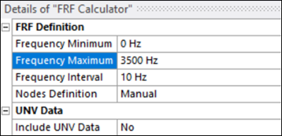
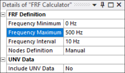
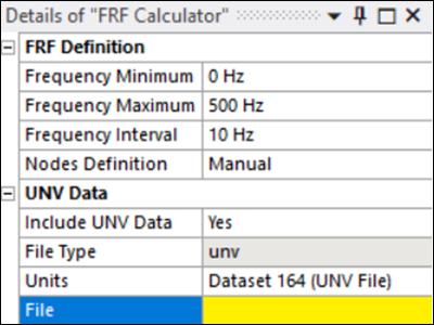
Set the Details for the FRF Calculator object as shown below. This frequency range (0 – 3500Hz) is chosen to account for the first six eigenvalues for this case.
Note that in this tutorial you are going to manually define the node pairs (in Step 6). Instead of node definition, you can choose the option for output and input nodes to populate the FRF Worksheet. Refer to the Node Definitions section in the FRF Calculator Details documentation for more information.
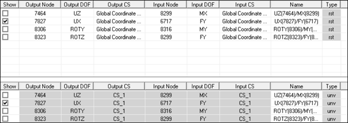
Populate data in the FRF Worksheet.
Add node pair data to the FRF worksheet:
Right-click in the worksheet and a row for a DOF pair.
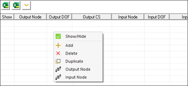
Observe that it shows details as below:
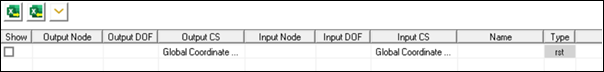
Select the cell below the Output Node header and add mesh node
7687(this can be this can be selected using keyboard hotkey m in the geometry window and then selecting using the ID as below).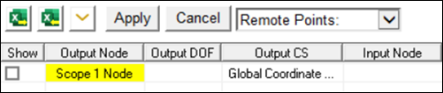
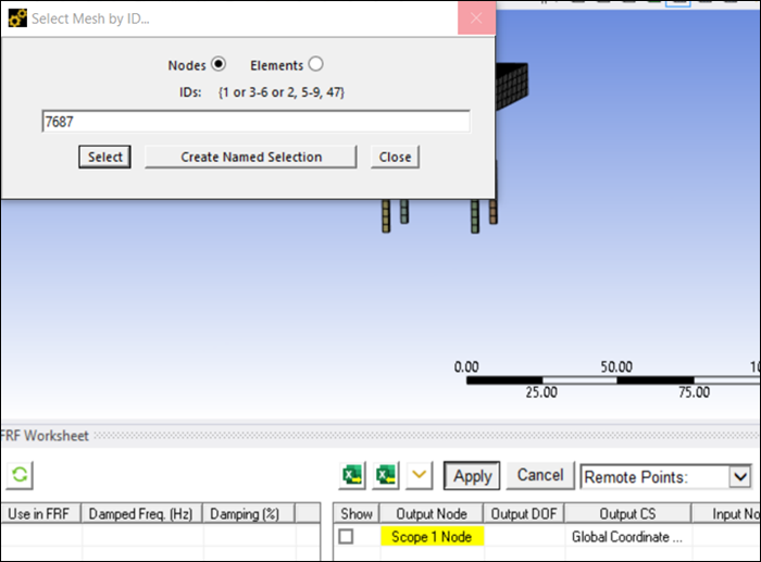
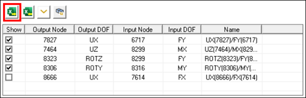
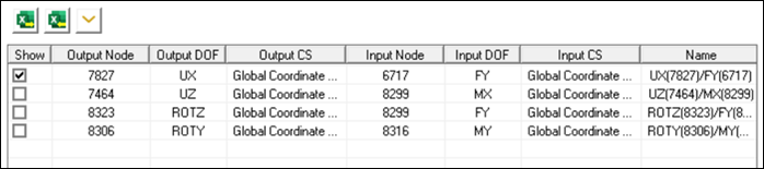
Define details as shown below for the first row and select the Show check box.

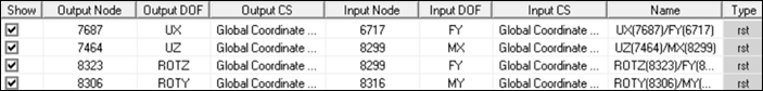
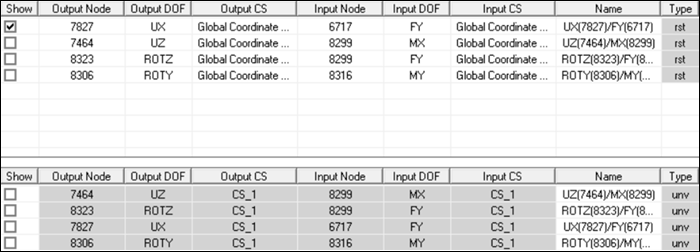
Define the FRF Worksheet rows shown below using the and right-click options. Refer to the FRF Worksheet documentation for more details.
Optional steps:
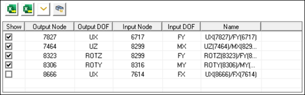
Add another row in the worksheet. Add an output or input node using the Remote Points drop-down menu as shown in the figure below and click to scope the node at the remote point (node ID
8666in this case).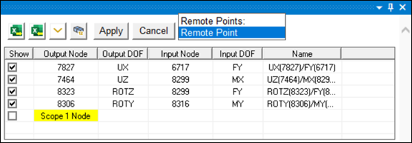
Export the worksheet to an Excel file using the button as highlighted below (an exported worksheet is available in the tutorial input folder).
You can also use the option of importing a worksheet from Excel to populate the node pair data in the FRF Worksheet table instead of adding it manually as described in steps 6a to 6e. Note that the data in the Excel file should be in a specific format as described under Import Worksheet from Excel in the FRF Worksheet documentation.
Delete the row added in the first optional step above.
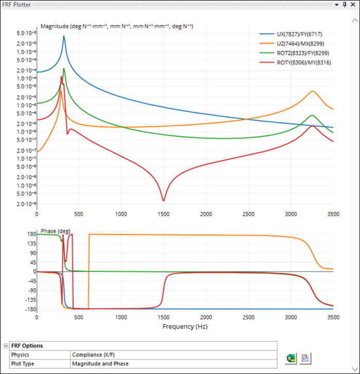
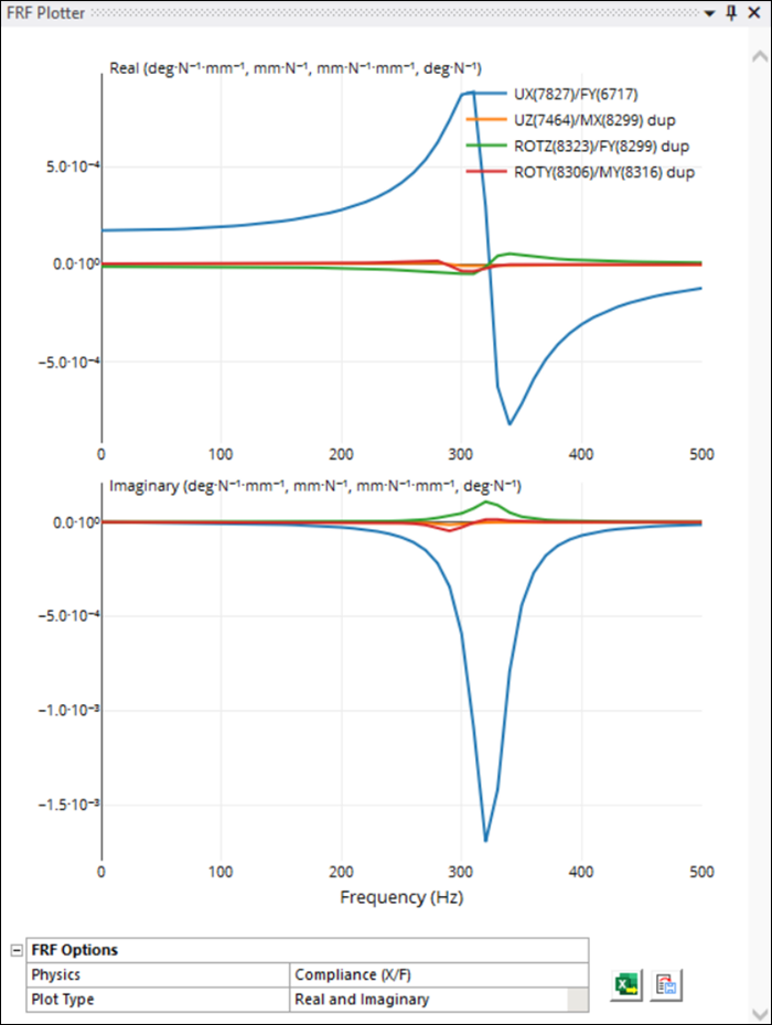
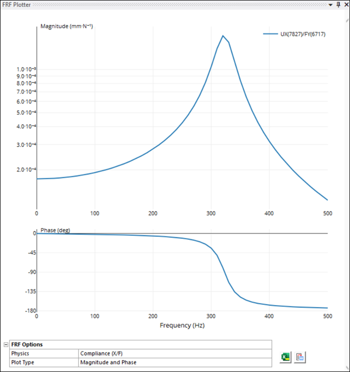
Generate the FRF Calculator and observe that the FRF Plotter appears with the plots shown below for four DOF pairs showing values. The peaks here indicate the presence of the natural frequencies of the structure. The magnitude and phase of multiple FRFs on a structure are used to determine the mode shape.
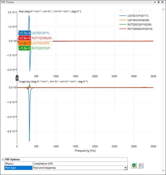
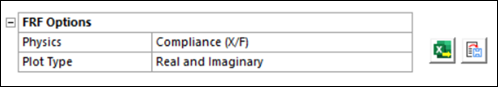
Change the Plot Type to and confirm that you see the plot shown below. Any function that has amplitude and phase can also be transformed to real and imaginary terms. After transforming the FRF from Amplitude & Phase to Real & Imaginary:
The real part of the FRF will equal zero at natural/resonant frequencies.
The imaginary part will have peaks either above or below zero which indicate resonant frequencies. This is clearly evident from the plot below.
In addition to the Plot Type, you can toggle between different Physics types to plot , or curves. For example, is a measure of how much a structure moves (displacement, X) for a unit input of force (F). and are other common ways to display the FRF. uses units of velocity over force, whereas uses units of acceleration over force. Refer to the FRF Calculation Method documentation for more mathematical details on these options.
Change the frequency range in the Details panel for the FRF Calculator as shown below and observe that the change is reflected in the plots.
Export FRF Data in CSV and UNV Formats
Export the FRF Plotter data using the file option shown below and observe that it is exported as a .csv file and contains FRF data for all DOF pairs for all frequency intervals.
Now export the FRF Plotter data using the file option (see the FRF Worksheet documentation for more information).
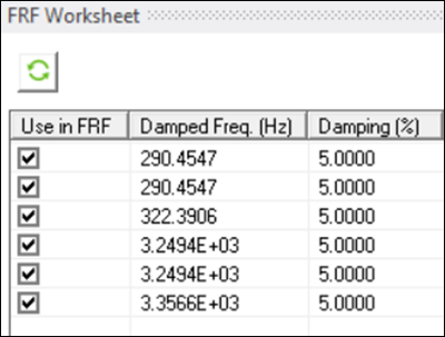
Change the Damping (%) from 2.0 to 5.0 in the FRF Worksheet Table 1 (Frequency Table) and the FRF Calculator.
Uncheck all rows in FRF Worksheet Table 2 (DOF Pairs – rst type) except the first and observe that the FRF Plot is available only for first DOF pair which shows magnitude and phase vs frequency.
Import FRF data and compare the plots
In the Details panel for the FRF Calculator, set Include UNV Data to and confirm that the File Type property is set to and that the FRF Calculator is undefined.
Import the unv file that was exported in Step 8b. Confirm that details shown below are available in the FRF Worksheet showing unv node data in Table 3 (DOF Pairs – unv type).
The unv model can be oriented using one of the three options: , or . In this tutorial, you have used the default option. For more details refer to the Orient By section under UNV Data in the FRF Calculator Details documentation.
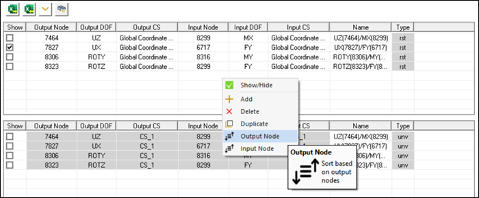
Sort the worksheet data in both worksheets based on output node IDs, by right-clicking in both worksheets and selecting (see below).
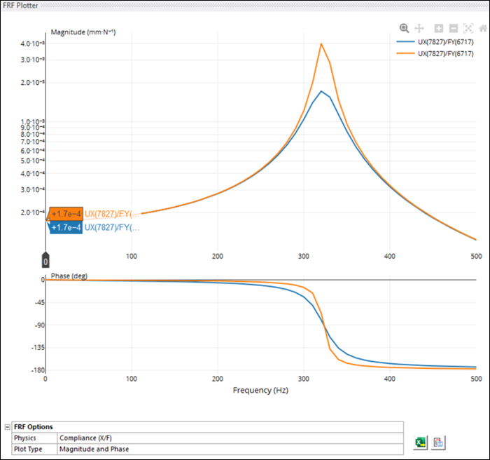
Select row number 2 in the unv data worksheet and compare the FRF plots between the two datasets with different Damping (%) values. You can see the difference between the peak at the resonant frequency drops for higher damping values. Also, the damping is proportional to the width of the peaks. The wider the peak, the heavier the damping.
Try selecting different rows in the FRF Worksheet to plot and compare data for different node pairs. Change the Physics and Plot Type and observe the changes.
You have completed the Frequency Response analysis and accomplished the overall objective for this tutorial.
Congratulations! You have completed the tutorial.