


| Analysis Type | Pre-Test Calculator |
| Features Demonstrated | NVH Toolkit Add-on, NVH toolkit system, PT calculator, sensor definition options, exciter definition options, analyze sensor mass effect |
| Licenses Required | Ansys Mechanical Premium/Enterprise/Enterprise PrepPost |
| Help Resources | NVH Toolkit Add-on |
| Tutorial Files | NVHPreTest.zip |
The tutorial guides by following topics:
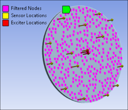
The Pre-Test Calculator introduces a result in the project tree that identifies optimum sensor and exciter locations for vibration tests for a given set of nodes filtered after user-selection.
The Pre-Test Calculator employs the Effective Independence Method (EIM) to identify the optimum location to place sensors. The method is based on the assumption that the optimum location for sensors is the one that ensures that the measured mode shapes are distinguishable from each other and provides good signal strength. Refer to Sensor Identification Method in the NVH documentation for more details about this method.
The Pre-Test Calculator employs the Driving-Point Frequency Response Function (DPFRF) method to identify the optimum location to place exciters. The method is based on the assumption that the optimum location for exciters is the one that ensures higher peaks in its Driving Point FRF, and therefore enhances the resonance of the structure. Refer to Exciter Identification Method in the NVH documentation for more details about this method.
Data files for this tutorial can be found here on the Ansys customer site.
The zip folder contains the following files:
PT_Model_Addon_Unsolved.wbpz - this is the input model that you will set up in the steps below. Copy this file to a working folder and complete the worked example.
PT_Model_Addon_Completed.wbpz - this is an example of the completed model once all the steps have been followed.
Start Workbench, and select > .
Browse to the working folder and select PT_Model_Addon_Unsolved.wbpz.
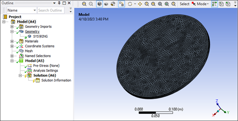
This Workbench project contains the Modal analysis system.
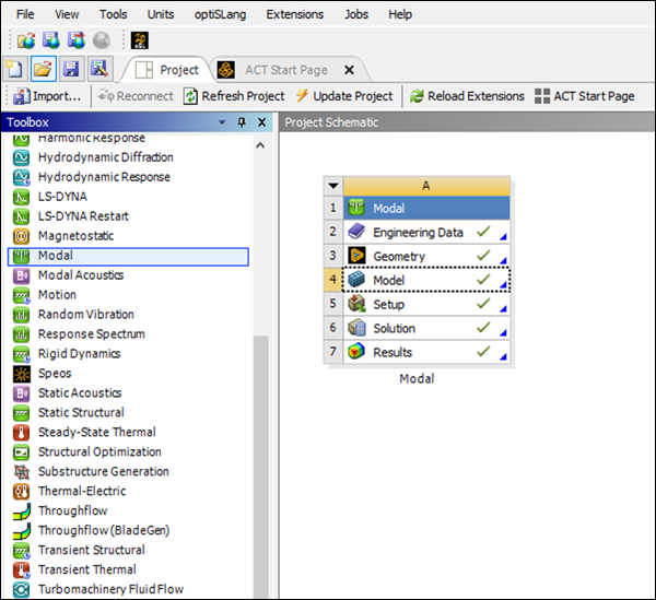
Double click the Model cell to open Mechanical.
To make the NVH Toolkit capabilities available, click the icon in the ribbon.
The icon is highlighted in blue, indicating that the add-on is loaded.
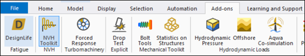
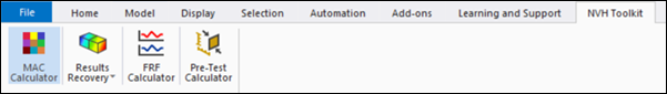
Once the add-on is loaded, the Ansys NVH Toolkit ribbon is visible, exposing all the NVH capabilities.
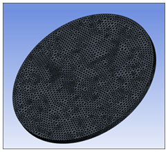
Verify geometric model
The geometry consists of a solid body, as shown in the figure below.
Solve modal analysis
To verify that the object is fully defined, right-click the Model or Solution and solve the analysis.
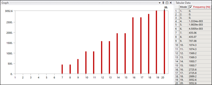
Verify the natural frequencies or eigenvalues (see below).
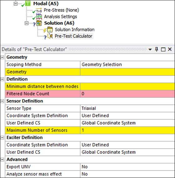
Right-click the Modal solution and insert a result. Confirm that it is in an undefined state with default Details as shown below.
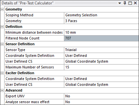
Go to the Geometry section and select the following three faces from the geometry view (one from the front view and another two from the rear, avoiding thick faces):
Click the button.
Go to the Minimum distance between nodes property and set a value of
1 mm. The initial candidate set of nodes for sensor and exciter locations will have a minimum distance of 1 mm, no nodes in free edges, no nodes in contact regions and no mid-side nodes. Observe that you get the following filtered nodes: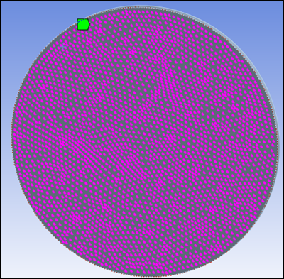
Notice that a new Named Selection has been created and the Filtered Node Count now contains
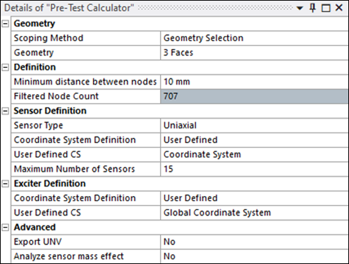
5379nodes.Change the Minimum distance between nodes property to a value of
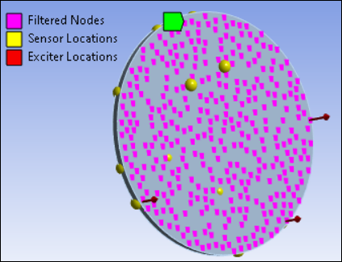
10 mm.Observe that you get the following result:
You can select the Coordinate System Definition for sensors and exciters. The option automatically computes a Coordinate System according to the Automatic Coordinate System Definition.
The option triggers the presence of the User Defined CS property defined below. The modification of this property affects all sensors and exciters that have already been found and that are displayed in the Pre-Test Worksheet.
It is possible to redefine the CS Definition in the Pre-Test Worksheet for each sensor/exciter.
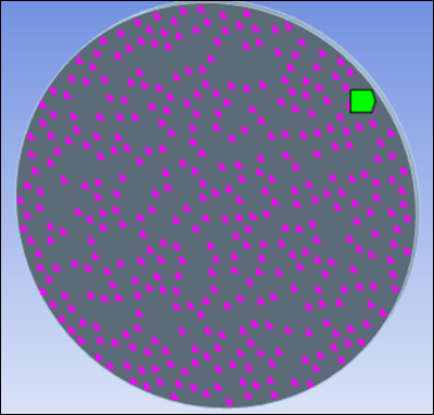
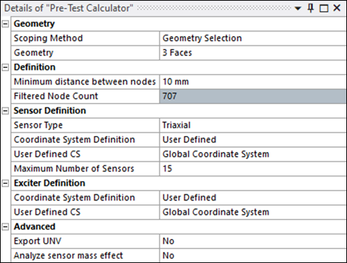
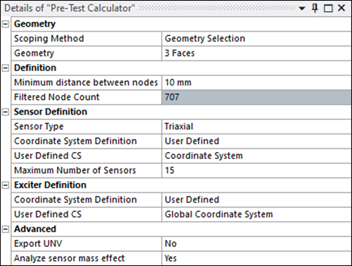
In the Details panel for the Pre-Test Calculator, set the properties shown below:
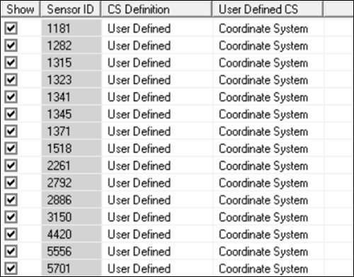
Observe that you get the following results from the Pre-Test Worksheet (in DPFRF Options, change Number of Exciters to
3):
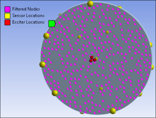
The front and rear view should appear as shown below:
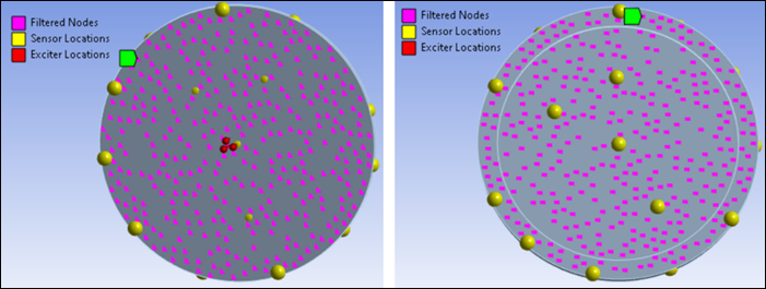
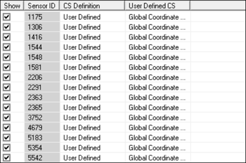
Check the results for the Sensors AutoMAC table by clicking the button at the bottom:
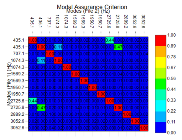
Note that almost all off-diagonal values are very low. This ensures that the measured mode shapes are distinguishable.
Change the Sensor Type to :
Observe you get the following results:
Front view:
Check results for the Sensors AutoMAC table:
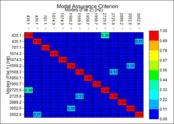
Note that almost all off-diagonal values are very low.
Set the following properties in the Details panel for the Pre-Test Calculator:
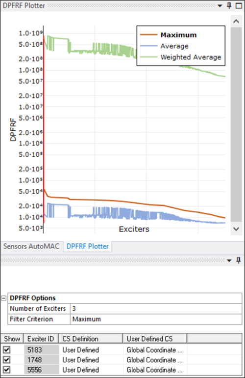
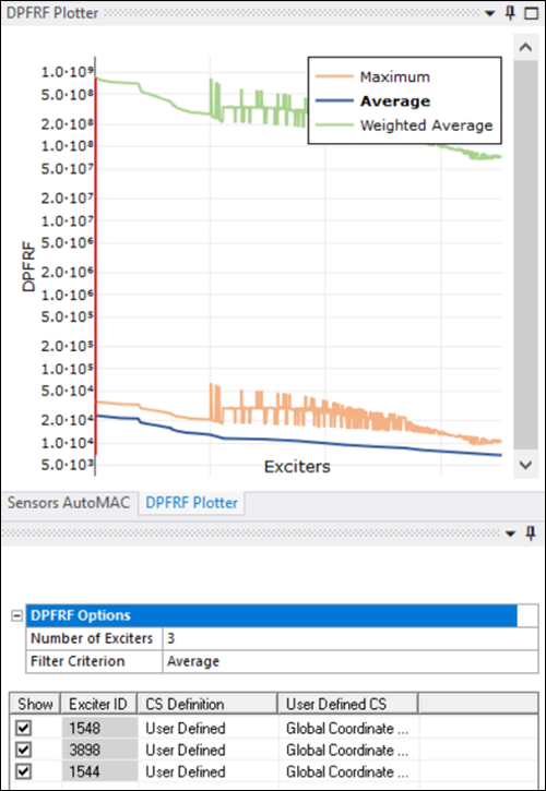
Set the following DPFRF Options:
Number of Exciters =
3Filter Criterion =
Check the following results in the DPFRF Plotter:
Front view:
This option takes the maximum of the DPFRF peaks. This is an indicator of the maximum strength of the response.
Finally, the candidate nodes are sorted according to this metric and the first nodes are considered the best exciters.
Under DPFRF Options, change the Filter Criterion to :
Front view:
This option takes the average of the DPFRF peaks. This is an indicator of how well the response covers all of the frequency range. For example, in this case it can be observed (see the previous tutorial step) how a candidate set of nodes exhibits a large maximum for a given mode but resonates poorly for the rest of them, showing bad coverage in the majority of the frequency range.
Finally, the candidate nodes are sorted according to this metric and the first nodes are considered the best exciters.
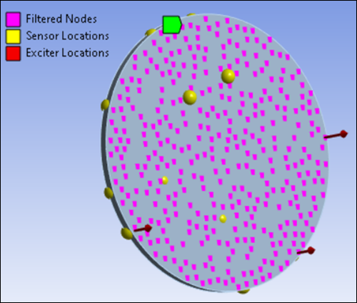
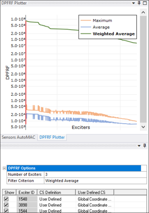
Under DPFRF Options, change the Filter Criterion to :
Front view:
This option takes the weighted average of the DPFRF peaks. The multiplication of both previous metrics.
Finally, the candidate nodes are sorted according to this metric and the first nodes are considered the best exciters.
Set the following properties in the Details panel for the Pre-Test Calculator:
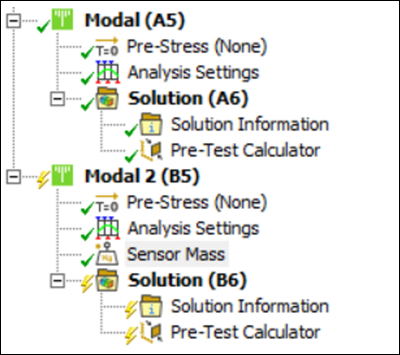
Then Generate the Pre-Test Calculator object.
Notice that a new Modal analysis has been created. It is duplicated from the first Modal analysis, with the same objects and a Sensor Mass load.
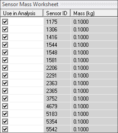
The Definition Method in Mass Definition properties can be set to either (using the same mass for all sensors) or (which allows you to select a different mass value for each sensor).
Select the method and set a Sensor Mass value of
0.1 kg.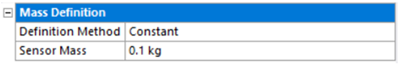
Observe that you get the following results in the Sensor Mass Worksheet.
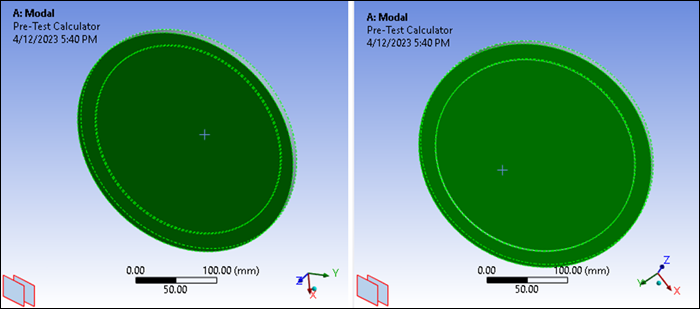
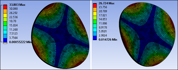
the analysis and compare results from the Modal analysis without Sensor Mass (left) and with Sensor Mass (right):
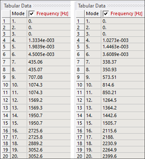
Note that natural frequencies have decreased because of the Sensor Mass, as expected.
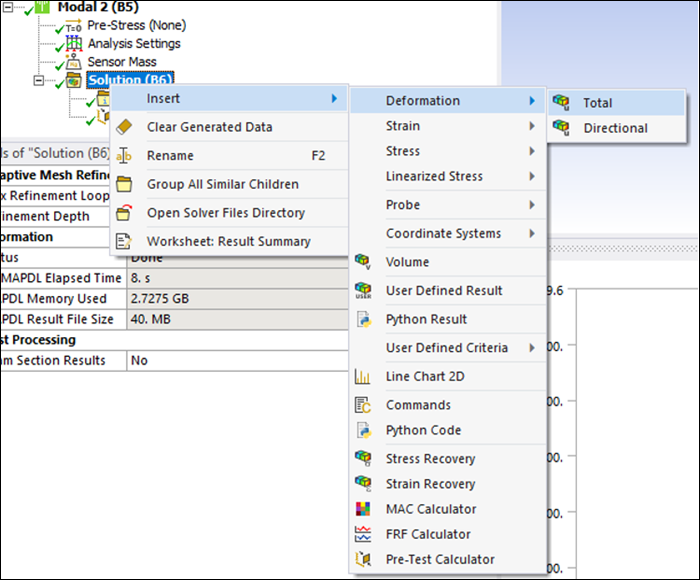
Right-click the Solution tree element for both Modal analyses, and select Deformation > to add a Total Deformation result.
Compare the results by right-clicking mode number 7 for each and selecting .
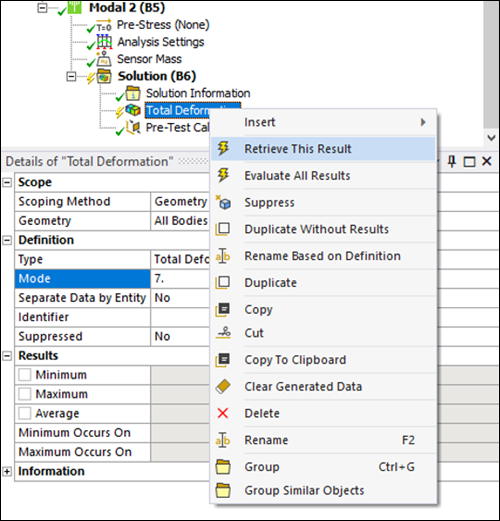
Compare the results and note that there are some slight differences:
You have completed the Pre-Test Calculator analysis and accomplished the overall objective for this tutorial.
Congratulations! You have completed the tutorial.