Any mesh-dependency of the KH-RT breakup model is mainly due to the
calculation of the liquid-gas relative velocity  in Equation 6–23
, in which
in Equation 6–23
, in which  is taken to be the CFD cell gas velocity. In Ansys Forte, the unsteady gas jet
model [[2]
, [77]
, [106]
] is used to remove this mesh-size dependency for
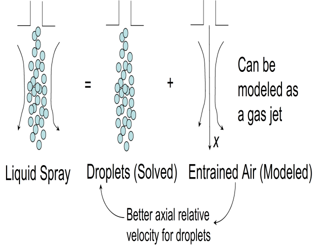
the liquid droplet-ambient gas coupling. The gas-jet model is based on unsteady gas-jet theory
[1], in which the
axial droplet-gas relative velocity is modeled without use of discretization on the CFD mesh
(Figure 6.4: Unsteady gas-jet model
).
is taken to be the CFD cell gas velocity. In Ansys Forte, the unsteady gas jet
model [[2]
, [77]
, [106]
] is used to remove this mesh-size dependency for
the liquid droplet-ambient gas coupling. The gas-jet model is based on unsteady gas-jet theory
[1], in which the
axial droplet-gas relative velocity is modeled without use of discretization on the CFD mesh
(Figure 6.4: Unsteady gas-jet model
).
In the gas-jet model, the jet tip develops with respect to time according to:
 | (6–43) |
where x is jet tip penetration, y is the local spray-axial location of the particle, K is an entrainment constant, U inf,eff is the "effective injection velocity", d eq is the equivalent diameter which is related to nozzle diameterD and liquid-gas density ratio by:
 | (6–44) |
The downstream spray-axial location x 0 marks the start of jet-velocity decay and is calculated as:
 | (6–45) |
The effective injection velocity is determined as an integral of the response to changes of the injection speed from the start of injection t 0 to the current time t :
 | (6–46) |
The response function R takes the form:
 | (6–47) |
where  is a response time scale, which is related to the local flow time scale
 by a Stokes number:
 | (6–48) |
This assumption is justified by the fact that a fluid particle responds to a change in the surrounding gas velocity exponentially [19] . The time scale of the response is determined by how long the local fluid particle has resided in the flow and by the local spray-axial location of the particle (denoted as y ).
The local gas-jet speed along the spray-axis direction is correspondingly calculated as:
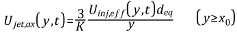 | (6–49) |
Assuming axis symmetry, the gas-jet velocity at any radial location r within the jet cross-section can be calculated as [2] :
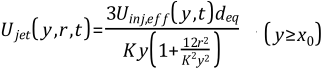 | (6–50) |
Using the gas-jet velocity in Equation 6–50
, the droplet-gas relative motion is
modeled as:
where  is the droplet velocity vector, CD is the drag
coefficient,
is the droplet velocity vector, CD is the drag
coefficient,  is the local gas-phase turbulent fluctuating velocity vector, and
 is acceleration due to gravity.
  is the gas-phase mean flow velocity with the axial component corrected by
Equation 6–50
. The radial and
azimuthal components are retained, so that other flow velocity components are not
influenced.
is the gas-phase mean flow velocity with the axial component corrected by
Equation 6–50
. The radial and
azimuthal components are retained, so that other flow velocity components are not
influenced.
The gas-jet-corrected relative velocity Urel :
 | (6–51) |
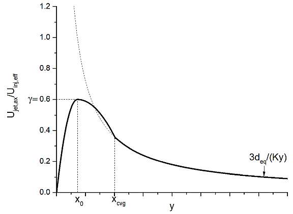
only applies beyond a distance x0 from the nozzle. In the near-nozzle region (y < x0 ), where the droplet velocity is very close to the injection velocity, a parabolic profile is used, which merges with the profile for y > x0 (see Figure 6.5: Jet velocity profile in the unsteady gas-jet model ), such that the jet velocity is:
 | (6–52) |
in which  is a constant with a fixed value of 0.6. Applying the parabolic entrained
gas-jet velocity profile along the spray axis is very effective in reducing the mesh-size
dependency of the breakup models.
is a constant with a fixed value of 0.6. Applying the parabolic entrained
gas-jet velocity profile along the spray axis is very effective in reducing the mesh-size
dependency of the breakup models.
In Ansys Forte, the Gas Entrainment Constant K in Equation 6–43 is a user-defined input. A larger value of K promotes gas entrainment and thus reduces spray penetration length.