


This section is arranged in the following parts:
Units:
Pay special attention to units. Be sure you enter units correctly as specified for the case, and do all the conversions correctly or allow the Simulation Interface to convert values for you whenever possible.
These comments apply to using the Sector Mesh Generator  , which opens into its own window from the Geometry Editor
panel.
, which opens into its own window from the Geometry Editor
panel.
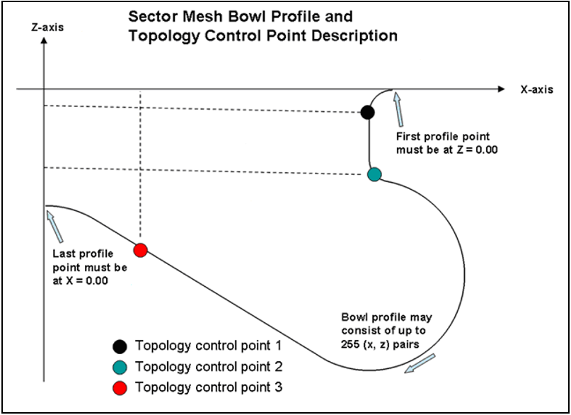
Obtain the bowl profile data. Sometimes these are given in the form of spline segments that have been extracted from CAD drawings or another mesh. You must order these coordinate points and then convert these to X, Z pairs. The X-Z coordinate frame must be defined as follows:
X is the radial direction from the center axis of the cylinder toward the cylinder wall (liner). A value of X=0 is at the cylinder center axis. At the cylinder wall, the value of X should be Bore/2.
Z is the vertical distance from the face of the piston lip in the direction of the cylinder head. The value of Z=0 must be at the outer edge of the piston face (closest to the cylinder wall). Z coordinates into the piston bowl will be negative.
The first point in the bowl profile should be the outer point on the piston face nearest to the cylinder wall (Z=0, X= Bore/2 - crevice_width). If the X coordinate is smaller than Bore/2 - crevice_width, the mesh generator will automatically extend the profile to this point. The actual first point will be set to (Z=0, X= Bore/2 - crevice_width).
If you have no information about the crevice, start with the default crevice values (1 cm long, 0.1 cm wide).
Note that the "crevice width" cannot be set to 0, even if the Include crevice volume option is unchecked. Similarly, the radial cell count corresponding to the crevice width cannot be 0. In other words, even if you do not want to include the crevice block, the topological block above the crevice must always be retained.
If you do not want to mesh the crevice volume, the Include crevice volume option should be unchecked, and the Axial cell count corresponding to the crevice volume should be set to 0.
Only include points that describe the profile from the piston face outer edge to the tip of the bowl at the center axis. Do not include points on the cylinder head.
The Sector Mesh Generator will assume a flat cylinder head. If this is not desired, you must generate the mesh using ICEM CFD or K3PREP, or consider using a 360° mesh instead of a sector mesh. Forte also is able to model sector engine geometry using Automatic Mesh Generation, which can also handle sector geometry with a non-flat cylinder head.
Once you have defined and saved the profile, the next step is to determine which topology is most appropriate for your profile. Look at the different topology options and select the one that looks the most like yours.
Determining Mesh Control Points and Size Parameters is an iterative trial-and-error process. The Mesh Control Point "fractions" are fractional distances along the entire length of the bowl profile. So if you think about stretching out the profile into a straight line and scaling it to a distance of 1.0, the control-point location parameters are the distance where each control point lies along this line, starting from the outer edge (Z=0, X=Bore/2-crevice_width). Make your best guesses, since it is easy and quick to iterate once you create an initial mesh. For example, for Topology #1, you might have 0.25,0.3,0.4, 0.7, for your starting locations for Control Points 1,2,3,4, respectively.
Cell counts are estimated based on trying to make the side size of any cell somewhere between 1 and 2 mm, where ~1.3 would be better for production runs, but ~2 might be better for initial setup verification (that is, the coarser mesh will run faster).
Use the Composition Calculator utility to calculate the following compositions:
Intake port/inlet composition for engine cases with valves and ports.
Exhaust port initial composition for engines cases with valves and ports.
In-cylinder initial composition at IVC for engine cases that are in-cylinder only.
The Composition Calculator can be accessed from the Utility menu or the Composition
Calculator  button on the toolbar. Refer to the
Forte User's Guide, for further
details of how to use the Composition Calculator utility.
button on the toolbar. Refer to the
Forte User's Guide, for further
details of how to use the Composition Calculator utility.
When high EGR is present and the engine is expected to generate a lot of NOx in the engine-out exhaust, then it may be necessary to adjust the initial gas composition to include some small fraction of NO in the initial conditions. This can be important as significant amounts of NO (that is, greater than ~50 ppm) can impact the ignition process through NOx-fuel sensitization effects. In addition, with high EGR, the presence of NOx in the exhaust can feed back to the overall measured exhaust of NO.
The molecular weight of NO (30 g/mole) is about the same as air or vitiated air (~29 g/mole). For this reason, adding 25 ppm (0.000025 mole fraction) of NO is approximately equivalent to adding 0.000025 mass fraction. For a more exact calculation, you would need to convert the mass fractions of the initial composition to mole fractions, add the ppm NOx, re-normalize, then convert back to mass fractions.
Ansys Forte requires the total mass of fuel injected, which is assumed to be per cylinder, and per cycle. In contrast, often the data available is per engine or per stroke. If data are provided per engine, then you need to divide by the number of engine cylinders for the input to Forte. If the data is provided per stroke, then the conversion is as follows:
If the per-stroke fuel data [mg/stroke] is given for one cylinder, then the Forte input is:

If the per-stroke fuel data [mg/stroke] is for the whole engine, that is, for a multi-cylinder engine, then the input to Forte is:

With IVC pressures and temperatures, there are typically uncertainties in these values. The temperature value is typically a derived value, based on the measured pressure, mass of air + EGR in the cylinder at IVC, and the ideal-gas relation. The pressure measured at IVC has higher uncertainty than the pressure measured after compression has begun, prior to fuel injection. For this reason, the standard procedure is to do one round of iteration to determine the pressure, as follows:
Use the given initial P and T and run the case to ~2 CA before start of injection.
Compare the predicted pressure profile up to this point with the measured values. If the pressure is too low or too high just before start of injection (SOI), adjust the IVC pressure value. However, this adjustment should be no more than ~3 PSI, which is less than ~0.2 bar.
Since the measured temperature is derived from the pressure and it is important to keep the total mass in the system consistent with measured values, also scale up the IVC temperature according to the adjustment made to pressure. In other words, if you change the initial pressure from 1.0 bar to 1.1 bar, also increase the initial temperature by a factor of 1.1 (that is, if it was 400 K, it should now be 440 K).
Possibly due to inadequacies of the surrogate-fuel model used, adjusting the injection timing as much as ~1 to 2 degrees CA to get reasonable timing for ignition is considered acceptable. The total mass of the fuel into the system, however, is accurately measured, as is the total air in the system, so these should not be adjusted. The main reason to make this adjustment is for comparison of emissions (in addition to ignition) with a focus on trends, rather than just seeking how well a particular mechanism provides ignition. Note that if you do not have the pressure trace close to agreement with experiment, there is little reason to compare emissions, because they will be at least as wrong as the pressure profile (which is an indicator of the temperature profile in the simulation).
The best way to judge the injection timing is to compare the heat-release rate (HRR) between prediction and experiment. Both are usually derived from the pressure trace, but this comparison shows more clearly the ignition timing than the pressure trace itself. The initial ignition behavior will be strongly dependent on the injection timing. The following adjustments may be acceptable:
If your heat-release peak is shifted by a couple of crank angle degrees relative to experiment, then you can shift the SOI of injection accordingly. This assumes that the width of the HRR curve is about the same as the data.
If the predicted HRR curve shows a higher peak and skinnier profile than the data, you might need to adjust the duration of injection (or, conversely, a low peak with an overly fat HRR may need a shorter duration.)
If there are multiple injection events, then this problem becomes more complicated. You may be able to see the HRR signature from the different injections, depending on how much heat is released as a result, but it may be hard to justify independently moving one peak relative to another or changing fuel splits. One would expect that the timing delay between actuator and fuel injection would not be different for different injection events, so the best approach would usually be to shift all events together.
In general, calibrating beyond the basics is not desirable. However, it is possible that some of the standard spray or turbulence parameters might need to be adjusted in the case of the engine conditions or fuel properties being outside of conventional heavy-duty diesel-engine operation. Only a few such parameters typically have noticeable impact on the results. The following provide some guidelines as to the effects to expect and the degree to which a parameter has an impact on the observed engine behavior. Here, the degree of the effect (High, Medium, Low) indicates the effect relative to other parameters listed. All of these parameters have a secondary, minor effect compared to the basic calibration described above. Note that while the Discharge Coefficient has the largest effect of these parameters, it may not be considered an "adjustable" parameter, if you have made some attempt to estimate it based on a nozzle-flow model, for example.
Table 4.1: Parameters providing secondary impacts on engine behavior
| Typical observed effect of increasing this parameter on: | |||||||
| Relative effect (H,M,L) | Parameter label | Recommended range | Default value | Physical effect of increase | Peak pressure | Expansion pressure | Ignition timing |
| H | Nozzle Discharge Coefficient | 0.7–1.0 | 0.7 | Decreases the injection velocity; increases initial droplet size. Effect on droplet size is typically dominant, which leads to slower vaporization rate, delayed ignition. | -- | Lower | Delayed; lower HRR slope |
| M to H | RT Distance Factor | 1.7–2.5 | 1.9 | Delays secondary breakup and therefore vaporization | -- | -- | Delayed |
| M | KH Time constant | 20–80 | 40 | Delays spray breakup near nozzle | -- | -- | Delayed; lower HRR slope |
| M | Entrainment constant | 0.3–0.7 | 0.5 | Enhances entrainment of air into fuel jet | Lower | Lower | Lower slope of HRR |
| M | Fuel droplet temperature (K) | 350–500 | 400 | Increases enthalpy of fuel jet | Increase | Increase | Earlier; Increase HRR slope |
| L | KH size constant | 1.0 | 1.0 | Delays spray breakup near nozzle | -- | -- | -- |
| L | RT size constant | 0.1–0.2 | 0.15 | Delays breakup away from nozzle | -- | -- | -- |
| L | RT time constant | 1.0 | 1.0 | “” | -- | -- | -- |
| L | Collision radius of influence | 0.2 | 0.2 | Collision model range | -- | -- | -- |
| L | Cylinder head temperature | -- | -- | Could reduce liquid on head | -- | -- | -- |
| L | Chemistry solver: DCC parameters | Defaults | 10 K, 0.05 phi | Resolution of clusters | -- | -- | -- |
| L | # Particles injected per nozzle hole | 2000–5000 | 2000 | Resolution of droplets | -- | -- | -- |
Ansys Forte will calculate the apparent heat-release rate automatically from the predicted pressure profile. This data is stored in the Forte solution file as Net HRR. In some cases, however, the experimental data provided only include the pressure measurement and not the derived heat-release rate. In other cases the heat-release rate is provided, but because there are some uncertainties in how that data was derived from the pressure profile, it may be better to calculate it so that the method is consistent with the model data and the comparison between simulation and experimental data is consistent.
The HRR profile can be calculated in Excel directly from the pressure vs. CA data, using the following formulation:

Here, Q is the heat-release, and
 is the heat-release rate, which is usually desired in J/degree
units. CA is the crank-angle,
is the heat-release rate, which is usually desired in J/degree
units. CA is the crank-angle,  is the specific heat ratio of the gas, which is taken to be
1.35, V is the in-cylinder volume, and
p is pressure. Note that Forte uses this
same formula in the calculation of the HRR in the
thermo.csv file.
is the specific heat ratio of the gas, which is taken to be
1.35, V is the in-cylinder volume, and
p is pressure. Note that Forte uses this
same formula in the calculation of the HRR in the
thermo.csv file.
If the volume of the chamber is not available, it can be calculated from the crank angle and engine parameters. First calculate the position of the piston, which will require the connecting-rod length (L) and the crank radius (R). Then, use that along with the engine Bore and the clearance volume to calculate the total volume in the cylinder at each crank angle. The calculations are as follows:
Piston position,
 is defined as follows:
Volume can then be calculated as:
At the first CA point: dQ=0
At CA point n, where n = 1, .., last:

Be careful with unit conversions! …It’s a good idea to compare the calculated volume profile with that calculated by Forte to make sure no mistakes have been made in steps 1 & 2.


Tip: You can create a placeholder thermo.csv in a folder that resides as a parallel-level directory to your run directory and put the CA vs. AHRR data into that file for direct comparisons during run-time using the Monitor plotting. For example, create a directory called xData_Run1 and place it in the same parent directory of the Run001 directory, then copy any thermo.csv file into the xData_Run1 folder, edit it and replace the CA, P, and AHRR columns with the experimental data (with the units expected in thermo.csv), but zero out all other columns. Now your plot will show your run-time comparison in the Monitor window.
Once you have the Pressure and HRR data in Excel, you can easily import it into the Ansys Forte Monitor for direct comparisons with predictions. First, create a separate sheet that has just the values of CA, P, V, and HRR in separate columns. Create column headers that indicate the label and give the units in Forte-recognizable unit-strings. These could be, for example:
Crank angle (deg)
Pressure (MPa)
In-cylinder volume (cm3)
Apparent heat release rate (J/deg)
With the columns of data set up in this way, save the sheet as a comma-separated-values text file (.csv) using Excel's "save as … other format" option and name it thermo.csv.
From the Ansys Forte Monitor, you can now read the data. To compare them against the simulated results, create an empty file named MONITOR and place it next to the newly modified .csv files. Group them in a folder and place it next to the Nominal folder of your simulation. Next, launch Forte Monitor and choose the working directory as the one containing the two sets of results. Allow the software to read the labels from the CSV file. It will parse the unit strings in parentheses and then will know the units context, so that conversions can be made using the Units Preferences options.
To make sure everything was set up correctly, always review the spray injection and vaporization behavior in a visualization tool, such as Ansys EnSight. Make sure that the injection timing aligns with the SOI/DOI values provided in the setup, and that the spray is pointed into the piston bowl.
For a "good engine" we'd expect the combustion to be taking place primarily in the bowl and that the droplets are getting consumed before they hit the wall. If spray seems to be impinging on the wall (undesirable) this could point to issues with the spray model, such as the discharge coefficient being too high, for example. If spray droplets are migrating out of the bowl and persisting into the expansion stroke, then the vaporization or fuel model may not be the best for this case. While it is possible these types of phenomena are real, it is good to first check whether inputs are reasonable and that the results are not sensitive to some estimated parameter.
Another good check is to confirm that the total mass of fuel injected, as reported at the end of the Forte log file, matches the value input in the spray injection data. This should be the total fuel injected for all nozzles (that is, not just the one nozzle represented in the sector), since that is what is measured and Forte takes care of the periodicity internally.
The emissions and engine-performance data can be found in summary form at the end of the FORTE.log file in the working directory of each run directory. Since these are single-point data, they are not otherwise accessible from a visualization tool. The Forte log contains the following example of summary data:
IMEP (Indicated Mean Effective Pressure)
ISFC (Indicated Specific Fuel Consumption)
Thermal Efficiency
Emissions indices for NOx, CO, UHC (unburned hydrocarbons), and soot, in the units of g/kg-fuel. These values are at the end of simulation, usually exhaust-valve opening, so they are engine-out conditions, not exhaust-system-out.
In addition, species emissions in the units of PPM can be determined from the molefraction.csv file found in the working directory of each parameter-study run. To get EVO emissions numbers, scroll down to the EVO crank angle (last row) and then go to the column for the molecule of interest. Note that the fraction of NOx is the sum of the fractions of NO + NO2. PPM is 106 times mole fraction.
Note that, for an in-cylinder-only simulation, the IMEP and ISFC are calculated based on integrating the P-V curve for the compression and expansion strokes (that is, -180 CA ATDC to 180 CA ATDC, where 0 CA ATDC is the firing TDC), which is different from what is measured. Typically, an in-cylinder-only simulation starts from IVC and ends at EVO. The P-V curve between IVC and EVO is integrated directly. The integrations for "-180 CA ATDC to IVC" and "EVO to 180 CA ATDC" are approximated. For example, the work for "EVO to 180 CA ATDC" is approximated as 0.5*(PIVC+PEVO)*(VEVO-VBDC), in which PIVC and PEVO are the pressures at IVC and EVO, respectively, and VEVO and VBDC are the volumes at EVO and BDC, respectively. Also, measurements are usually based on brake power, rather than indicated power. So it is expected for these to be approximate rather than an exact match, relative to the data. However, it is expected that the predicted results follow the correct trends.
In some cases, units of [g/hour] are preferred to the emission indices that are in units of [g/kg-fuel]. The conversion accounts for the fact that the total fuel injected into the engine system is "per cycle" and a cycle is two revolutions of the crank. As discussed in SAM Settings for Spray Vaporization, the fuel input to Forte is "per cylinder" and "per cycle." In this way, knowing the total fuel injected per cycle per cylinder and knowing the revolutions-per-minute speed of the engine as well as the number of engine cylinders, the units of [g/h] are obtained as follows:

where Revolution_per_cycle is 2 for a four-stroke engine and 1 for a two-stroke engine.