


You can review your results in the graphics window using objects such as contours, vectors, pathlines, particle tracks and XY plots. You can also create surfaces for further exploring the results.
These different postprocessing tools are discussed in the following sections:
You can create different types of surfaces to visualize your results, including points, lines, rakes, planes, and iso-surfaces.
Note: To ensure updated surface definitions (for example, if you change the location of a line) are properly shown when included in a scene or other graphics object, display the surface before re-displaying the containing object.
Refer to the following sections for more details:
You may be interested in displaying results at a single point in the domain. For example, you may want to monitor the value of some variable or function at a particular location. To do this, you must first create a "point" surface, which consists of a single point. When you display node-value data on a point surface, the value displayed is a linear average of the neighboring node values. If you display cell-value data, the value at the cell in which the point lies is displayed.
![]() Results → Surfaces
Results → Surfaces
![]() New → Point
New → Point
To create a point surface, use the Figure 4.115: Properties of a Point Surface.
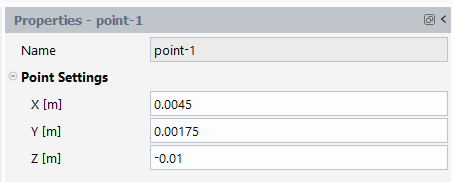
Here, you would typically set the Name, and the X, Y, and Z coordinates of the point.
See Point Properties for details.
A line is a straight segment that extends up to and includes the specified endpoints; data points will be located where the line intersects the faces of the cell, and consequently may not be equally spaced.
![]() Results → Surfaces
Results → Surfaces
![]() New → Line
New → Line
To create a line surface, use the Figure 4.116: Properties of a Line Surface.
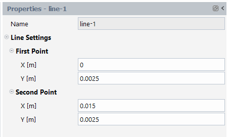
Here, you would typically set the Name, and various Line Settings, such as the X, Y, and Z coordinates of the First Point and the Second Point of the line surface.
See Line Properties for details.
A rake consists of a specified number of points equally spaced between two specified endpoints.
![]() Results → Surfaces
Results → Surfaces
![]() New → Rake
New → Rake
To create a rake surface, use the Figure 4.117: Properties of a Rake Surface.
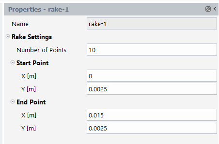
Here, you would typically set the Name, and various Rake Settings, such as the X, Y, and Z coordinates of the Start Point and the End Point of the rake surface.
See Rake Properties for details.
To display flow-field data on a specific plane in the domain, you will use a plane surface. You can create surfaces that cut through the solution domain along arbitrary planes.
![]() Results → Surfaces
Results → Surfaces
![]() Plane...
Plane...
To create a plane surface, use the Figure 4.118: Properties of a Plane Surface.
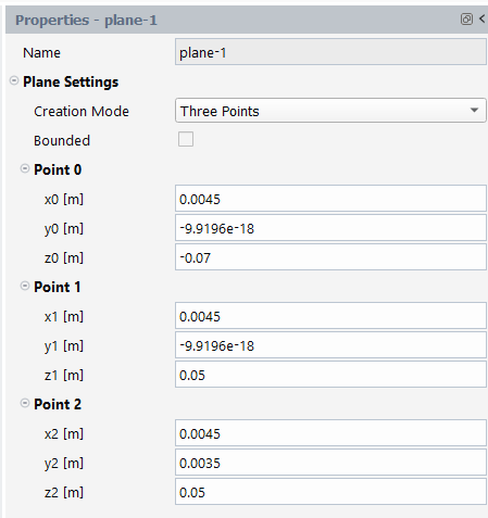
Here, you would typically set the Name, and various Plane Settings of the plane surface.
There are three types of plane surfaces that you can create (via the Creation Mode):
Coordinate system-based—the plane is created in the YX, ZX, or XY directions, bounded by the extents of the domain. You can move the plane to the desired location in the domain using the plane tool. For example, if you are using the YZ Plane method, you can drag the plane in the (+) or (-) X direction.
Point and normal—the plane orientation is determined by selecting a point and specifying a direction normal to that point. The extents of the plane are the edges of the domain. You have the option to control the orientation of the plane using the plane tool or you can compute the normal from a surface.
Three points—the plane orientation and extents are bounded by three points that you can select. You also have the option to manipulate the points and orientation of the plane directly in the graphics window using the plane tool.
See Plane Properties for details.
If you want to display results on cells that have a constant value for a specified variable, you will need to create an iso-surface of that variable. For example, generating an iso-surface based on x- , y-, or z- coordinate will give you an x, y, or z cross-section of your domain; generating an iso-surface based on pressure will enable you to display data for another variable on a surface of constant pressure. You can create an iso-surface from an existing surface or from the entire domain. Furthermore, you can restrict any iso-surface to a specified cell zone.
Important: Note that you cannot create an iso-surface until you have initialized the solution, performed calculations, or read a data file.
![]() Results → Surfaces
Results → Surfaces
![]() New
→ Iso-Surface
New
→ Iso-Surface
To create an iso-surface, use the Figure 4.119: Properties of an Iso-Surface.
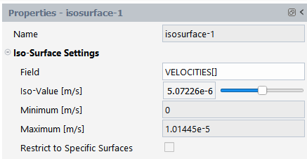
Here, you would typically set the Name, and various Iso-Surface Settings of the iso-surface.
Click at the bottom of the iso-surface properties panel to display the iso-surface in the graphics window.
Click at the bottom of the iso-surface properties panel to delete an iso-surface.
Instead of creating plane surfaces one at a time as described above, you have the option to create multiple plane surfaces at once using the Figure 4.121: Create Multiple Planes Dialog Box.
See Iso-Surface Properties for details.
Iso-clip surfaces are clipped surface that consist of those points on the selected surface where the scalar field values are within the specified range.
![]() Results → Surfaces
Results → Surfaces
![]() New
→ Iso-Clip
New
→ Iso-Clip
To create an iso-clip surface, use the Figure 4.120: Properties of an Iso-Clip Surface.
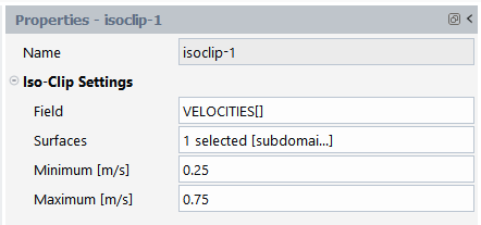
Here, you would typically set the Name, and various Iso-Clip Settings of the iso-clip surface.
Click at the bottom of the iso-clip properties panel to display the iso-clip in the graphics window.
Click at the bottom of the iso-clip properties panel to delete an iso-clip.
See Iso-Clip Properties for details.
Instead of creating plane surfaces one at a time as described above, you have the option to create multiple plane surfaces at once using the Figure 4.121: Create Multiple Planes Dialog Box.
![]() Results → Surfaces
Results → Surfaces
![]() Create Multiple Planes...
Create Multiple Planes...
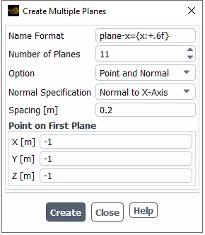
To use the Create Multiple Planes dialog box:
(Optional) Provide a format for naming the plane surfaces in the Name Format field.
Specify how many planes will be created in the Number of Planes field.
Select the method for how you want to create the planes in the Option drop-down list.
Point and Normal—similarly to the process described earlier in this section, you must provide a point and the direction normal to that point to define the first plane.
First and Last Point—you define the coordinates for the first and last point, which determines the orientation of the planes. The spacing is determined by how many planes you specify in the Number of Planes field.
(Point and Normal only) Specify the direction normal (perpendicular) to the plane in the Normal Specification drop-down list.
(Point and Normal only) Specify how far apart the planes are from each other in the Spacing field.
Provide the coordinate for the location of the first plane in the Point on First Plane group box.
(First and Last Point only) Provide the coordinates for the location of the last plane in the Point on Last Plane group box.
Click to create the new plane surfaces.
The new plane surfaces created using the Create Multiple Planes dialog box are added to the Outline View tree under the Surfaces branch and are now eligible for editing individually. Once created, the multiple planes cannot be edited as a group.
Instead of iso-surfaces one at a time as described above, you have the option to create multiple iso-surfaces at once using the Figure 4.122: Create Multiple Iso-Surfaces Dialog Box.
![]() Results → Surfaces
Results → Surfaces
![]() Create Multiple Iso-surfaces...
Create Multiple Iso-surfaces...
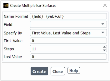
To use the Create Multiple Iso-Surfaces dialog box:
(Optional) Provide a format for naming the iso-surfaces in the Name Format field.
Select the field that you want to use for creating the iso-surfaces from the Field drop-down list. The availability of fields depends on the calculation. The following is a sample:
local shear rate—value of the local shear rate.
velocity-magnitude—magnitude of the velocity.
x-coordinate—value of the x-coordinate.
y-coordinate—value of the y-coordinate.
z-coordinate—value of the z-coordinate.
x-velocity—x-component of the velocity.
y-velocity—y-component of the velocity.
z-velocity—z-component of the velocity.
viscosity—value of the viscosity.
pressure—value of the pressure.
density—value of the density.
Specify the method you want to use for creating iso-surfaces in the Specify By drop-down list.
First Value, Last Value and Steps—using this method you must specify the First Value for the quantity that you selected in the Field drop-down list, specify how many iso-surfaces you want created by entering the number of Steps, and provide the final value for the selected quantity in the Last Value field.
First Value, Last Value and Increment—using this method you must specify the First Value for the quantity that you selected in the Field drop-down list, specify the size of the increments between the first and last value, which determines the number of iso-surfaces to be created, and provide the final value for the selected quantity in the Last Value field.
First Value, Increment and Steps—using this method you must specify the First Value for the quantity that you selected in the Field drop-down list, specify the size of the increments from the first value, and provide the total number of steps in the Steps field, which determines the total number of iso-surfaces to be created.
Last Value, Decrement and Steps—using this method you must specify the size of the decrement (negative increment) in the Decrement field, which will go backwards from the Last Value, provide the total number of steps in the Steps field, which determines the total number of iso-surfaces, and provide the final value for the selected quantity in the Last Value field.
Click to create the new iso-surfaces.
The new iso-surfaces created using the Create Multiple Iso-Surfaces dialog box are added to the Outline View tree under the Surfaces branch and are now eligible for editing individually. Once created, the multiple iso-surfaces cannot be edited as a group.
Static reports are available for computation of various postprocessing quantities.
![]() Results → Reports
→ New...
Results → Reports
→ New...
Once a report is created, click and the result is printed in the Console. Click and the result is saved to a file and location of your choice. Click and the result is printed in the Graphics window.
See Report Properties for details.
Reports can be printed in the workspace using the Print Report dialog box, accessible from the relevant report object property page.
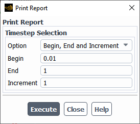
The following options are available when printing your reports:
- Timestep Selection
Indicate specific details of the time step (Current, First, Last, All, or specify the starting point, the ending point and a particular increment.
Reports can be saved in the workspace using the Save Report dialog box, accessible from relevant report object property page.
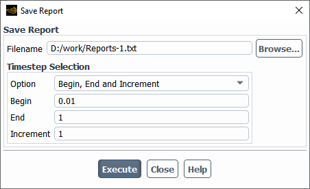
The following options are available when saving your reports:
- Filename
Specify the name and location of the report that you want to save.
- Timestep Selection
Indicate specific details of the time step (Current, First, Last, All, or specify the starting point, the ending point and a particular increment.
Reports can be plotted in the workspace using the Plot Report dialog box, accessible from relevant report object property page.
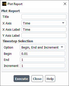
The following options are available when plotting your reports:
- Title
Specify the title you want to apply to the plot report
- X Axis
Specify the variable you want to apply to the x-axis for the plot report.
- X Axis Label
Specify the title you want to apply to the x-axis for the plot report.
- Y Axis Label
Specify the title you want to apply to the y-axis for the plot report.
- Timestep Selection
Indicate specific details of the plot report time step (Current, First, Last, All, or specify the starting point, the ending point and a particular increment.
Postprocessing graphics objects are available for visualizing the results of your simulation. You can display the mesh, contours, vectors, pathlines, and scenes. Scenes allow you to combine multiple graphics objects within a single graphics window.
Note: Only field variables that are appropriate and compatible for the specific workspace simulations are available in the Field dialog box.
Once you have created your graphics objects and/or made changes to their properties, you can:
Click to visualize the object in the graphics window.
Click to open the Save Image dialog box and proceed to save an image file of the object in the graphics window.
The available graphics objects are described in greater detail in the following sections:
The Line Integral Convolution algorithm allows you to integrate a vector over a part surface. It can be used to provide a uniform visualization of the flow of a vector over a surface. The settings used for drawing the LIC including the velocity field can be specified under LIC Settings in the Outline View.
![]() Results → Graphics
→ LIC Settings
Results → Graphics
→ LIC Settings
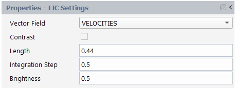
Line integral convolution can be drawn as part of contour objects or mesh objects in which faces are displayed. To draw LIC on a contour or mesh object, enable the option within their respective property panels as outlined in Mesh Properties and Contour Properties.
See LIC Settings Properties for details.
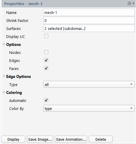
Mesh plots allow you to visualize and inspect the mesh.
To create a mesh plot, right-click Meshes in the Outline View tree and select New....
![]() Results → Graphics
→ Meshes
Results → Graphics
→ Meshes![]() New...
New...
Once you have made your property settings, click to visualize the object in the graphics window. You can also click to save an image file of the object in the graphics window.
See Mesh Properties for details.
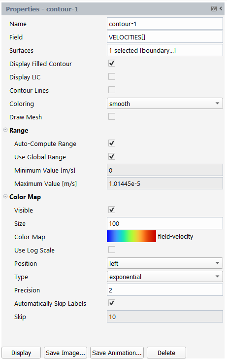
Contour plots are a valuable postprocessing tool that allow you to use color to represent the values of the specified field variable on the selected surfaces.
To create a contour plot, right-click Contours in the Outline View tree and select New....
![]() Results → Graphics
→ Contours
Results → Graphics
→ Contours![]() New...
New...
Once you have made your property settings, click to visualize the object in the graphics window. You can also click to save an image file of the object in the graphics window.
See Contour Properties for details.
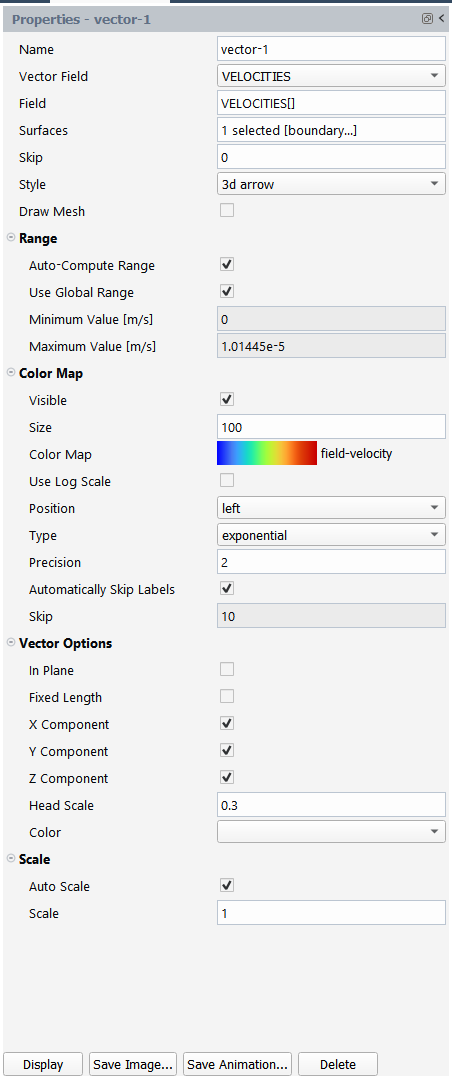
You can draw vectors in the entire domain, or on selected surfaces. By default, one vector is drawn at the center of each cell (or at the center of each facet of a data surface), with the length of the arrows represented by the selected vector field (typically the velocity) and the color of the arrows represented by the selected scalar field. The spacing, size, and coloring of the arrows can be modified, along with several other vector plot settings. Note that cell-center values are always used for vector plots; you cannot plot node-averaged values.
To create a vector plot, right-click Vectors in the Outline View tree and select New...
![]() Results → Graphics
→ Vectors
Results → Graphics
→ Vectors![]() New...
New...
Once you have made your property settings, click to visualize the object in the graphics window. You can also click to save an image file of the object in the graphics window.
See Vector Properties for details.
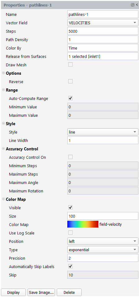
Pathlines are used to visualize the flow of massless particles in the problem domain. The particles are released from one or more surfaces that you have created as described in Surfaces. A line or rake surface (see Line Surfaces and Rake Surfaces) is most commonly used.
To create a pathline plot, right-click Pathlines in the Outline View tree and select New....
![]() Results → Graphics
→ Pathlines
Results → Graphics
→ Pathlines![]() New...
New...
Once you have made your property settings, click to visualize the object in the graphics window. You can also click to save an image file of the object in the graphics window.
See Pathlines Properties for details.
Use the Display Settings properties panel to change various attributes of the graphics window display.
![]() Results → Display
Settings
Results → Display
Settings
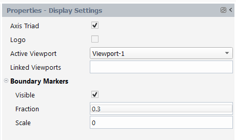
See Display Settings Properties for details.
Scenes can be used to display multiple graphics plots within a single window. For example, you could overlay contours of pressure across a valve with velocity vectors and the mesh at the same location. Scenes allow you to modify the transparency of each plot so that you can emphasize a particular plot or view.
To create a new scene, right-click Scenes in the Outline View tree and select New....
![]() Results → Graphics
→ Scenes
Results → Graphics
→ Scenes![]() New...
New...
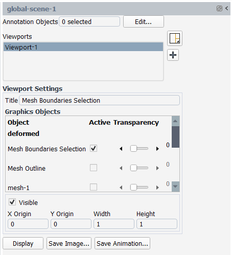
(Optional) Enter a Title for the scene.
Under Graphical Objects, select whether or not to include graphics objects in a scene by enabling or disabling the Active check box for the corresponding Object in the list.
Set the transparencies for the selected graphics objects by clicking the Transparencies field.
Once you have made your property settings, click to visualize the object in the graphics window. You can also click to save an image file of the object in the graphics window, or click to save an animation.
Animations can be saved in the workspace using the Save Animations dialog box, accessible from relevant graphics objects (contours, vectors, etc.).
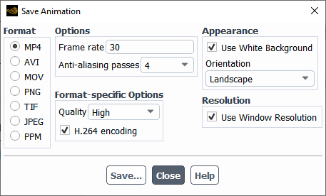
The following options are available when saving your animations:
- Format
Allows you to specify the saved animation format as either MP4 (default), AVI, MOV, PNG, TIF, JPEG, or PPM.
- Options
Contains general animation options.
- Frame rate
Specify rate of the frames (in frames per second, fps) to be set for the animation to be recorded. Generally, the default is 30fp (for MP4, AVI, or MOV formats).
- Anti-aliasing passes
Specify the number of anti-aliasing passes required to smooth out edges and distortions.
- Format-specific Options
Contains options that are specific to the chosen animation format.
- Quality
(MP4) Allows you to control the quality and resolution for the animation sequence.
- H.264 encoding
(MP4) Allows you to control the encoding for the animation sequence.
- Bit rate
(AVI and MOV) Allows you to control the bit rate for the animation sequence.
- Compression
(AVI, PNG, TIF) Allows you to control the compression method for the animation sequence.
- JPEG Quality
(JPEG) Allows you to control the compression rate (0-100) for the animation sequence.
- PPM Format
(PPM) Allows you to save the animation files as Binary (Default) or ASCII.
- Appearance
Specifies the general look of the saved animation.
- Use White Background
Allows you to save animations with a white background and a black foreground.
- Orientation
Controls the orientation of the animation as either Landscape or Portrait
- Resolution
- Use Window Resolution
Uses the resolution of the current graphics window when the image is saved.
Mirror planes allow you to define a symmetry plane for a non-symmetric domain for use with your graphics objects.
To use mirror planes, open the Results tab of the Ribbon and, under Graphics, select Mirror Planes... to open the Mirror Planes dialog.
![]() Results → Graphics
→ Mirror Planes...
Results → Graphics
→ Mirror Planes...
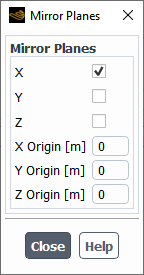
Specify whether the mirror plane will be oriented in the X, Y, or Z plane(s).
Specify the distance from the origin in the x, y, or z directions Use the X Origin, Y Origin, or Z Origin fields.
You can visualize your changes as you make them in the dialog, and adjust the settings accordingly.
You can assign specific materials to specific surfaces in your simulation.
To use material assignments, open the Results tab of the Ribbon and, under Graphics, select Material Assignment... to open the Assign Material To Surface dialog.
![]() Results → Graphics
→ Material Assignment...
Results → Graphics
→ Material Assignment...
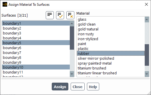
Specify one or more surfaces from the Surfaces list.
Specify a material from the Material list.
Click Assign to assign the selected material to the surface(s).
Postprocessing plot objects are available for visualizing the data from the results of your simulation. You can display the standard XY plots, or specialized plots for transient simulations.
The available graphics objects are described in greater detail in the following sections:
XY plots are a valuable postprocessing tool that allow you to plot variables related to your simulation.
To create an XY plot, right-click XY Plots in the Outline View tree and select New....
![]() Results → Plots
→ XY
Plots
Results → Plots
→ XY
Plots![]() New...
New...
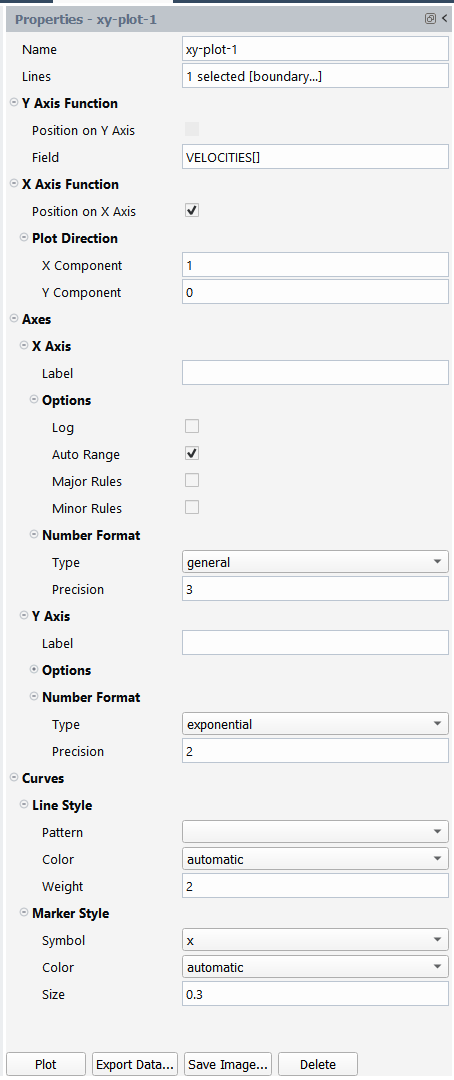
Once you have set your properties:
Click to display the plot in the graphics window.
Click to save the plot in another format.
Click to save the plot as an image.
Click Delete to remove the plot.
See XY Plot Properties for more details.
Transient plots are a valuable postprocessing tool that allow you to use study time-dependant aspects of your simulation.
To create a transient plot, right-click Transient Plots in the Outline View tree and select New....
![]() Results → Plots
→ Transient
Plots
Results → Plots
→ Transient
Plots![]() New...
New...
Once you have set your properties:
Click to create a hard copy of the plot.
Click to display the plot in the graphics window.
Click to save the plot in another format.
Click Delete to remove the plot.
Click to save the plot as an image.
Click to pick and choose the reports files that your plot is comprised of.
See Transient Plot Properties for more details.