


This chapter describes the fluid models available in Fluent Materials Processing, including details about the related material data parameters for each.
The proper selection of a fluid model is one of the most important aspects in the simulation of a flow. You need to always consider both the fluid and the flow. A particular constitutive equation is valid for a given fluid in a given flow.
To determine an appropriate model for your problem, you need to first collect as much data as possible about the fluid properties. Typical information includes the following:
Steady viscometric properties (shear viscosity
 and first normal-stress difference
  ). These data characterize the fluid in the presence of
large deformations.
). These data characterize the fluid in the presence of
large deformations. Oscillatory viscometric properties (storage and loss moduli
 and
and  ), also known as linear viscoelastic data because they
correspond to small deformations.
), also known as linear viscoelastic data because they
correspond to small deformations. Elongational viscosity. Although obtaining data on elongation is difficult and not very frequent, knowledge of the elongational viscosity can be of interest if the process involves a visible elongation component, for example, fiber spinning. This may be useful in choosing the appropriate constitutive equation and estimating the values of the various parameters.
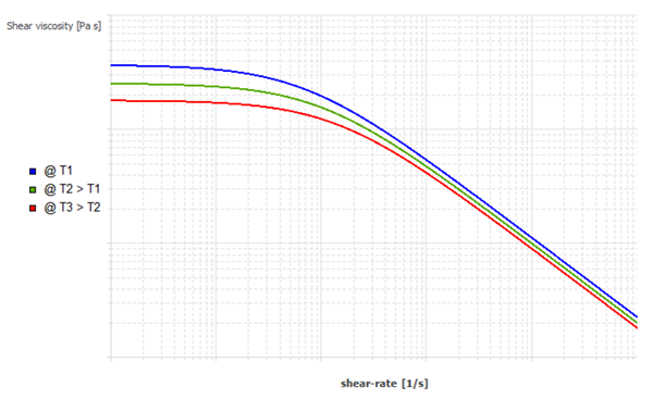
These data are not enough to evaluate the relevance of viscoelasticity in a given process. It is also necessary to characterize the flow itself and compare a characteristic time of the material to a characteristic time of the flow. In many situations, the flow can be characterized by a typical shear rate, which can be understood as a wall shear rate in a region of high gradients. For example, in a fiber-spinning process, a typical shear rate will occur at the wall in the vicinity of the die exit. In a contraction or expansion flow (for example, Figure 4.123: Contraction and Expansion Flow), consider the shear rate in the narrow section.
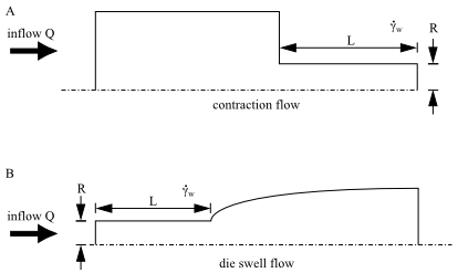
In a planar flow (Figure 4.123: Contraction and Expansion Flow a),
 | (4–24) |
where  is a typical distance.
In an axisymmetric flow (Figure 4.123: Contraction and Expansion Flow b),
 | (4–25) |
where  is a typical radius.
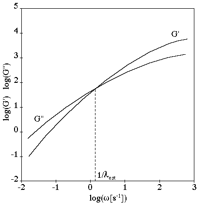
You also need to determine the elasticity level of the fluid. This can be
accomplished by evaluation of the fluid’s characteristic relaxation time.
When the oscillatory functions  and
and  are available, their intersection (occurring at a shear rate
 , as shown in Figure 4.124: Storage and Loss Moduli Curves) is often a reasonable choice for selecting a typical
relaxation time. Indeed, flows characterized by a typical shear rate lower than
, as shown in Figure 4.124: Storage and Loss Moduli Curves) is often a reasonable choice for selecting a typical
relaxation time. Indeed, flows characterized by a typical shear rate lower than
 are essentially dominated by viscous forces, while
viscoelastic effects may play an important role in flows characterized by a
shear rate higher than
are essentially dominated by viscous forces, while
viscoelastic effects may play an important role in flows characterized by a
shear rate higher than  .
.
Note that, due to the technological limitations of some rheometry equipment, it is not always possible to obtain viscoelastic data in the range of shear rates (or angular frequencies) where the process operates. In this case, your only option is to extrapolate experimental data for higher shear rates or angular frequencies. The selection of a particular model for such a case will be more qualitative.
A typical dimensionless number used to estimate the viscoelastic character of
a flow is the Weissenberg number  , which is the product of the relaxation time
  and a typical shear rate
  :
:
 | (4–26) |
When  is low, generalized Newtonian models are sufficient to
describe the flow; only at higher values of
is low, generalized Newtonian models are sufficient to
describe the flow; only at higher values of  are viscoelastic models required to characterize memory
effects.
are viscoelastic models required to characterize memory
effects.
Note that the Weissenberg number is probably not the best indicator for
viscoelastic models with several relaxation times or if there is shear thinning
in the flow. In such cases, a useful dimensionless number is the recoverable
shear  , defined as the ratio of the first normal-stress difference
 to twice the steady shear stress
  :
:
 | (4–27) |
The recoverable shear  gives the level of elasticity of a flow: if
  >1, the viscoelastic character of the flow is important, and
a viscoelastic model is required.
>1, the viscoelastic character of the flow is important, and
a viscoelastic model is required.
The different fluid models are studied in different flows described in Rheological Properties.
Steady Simple Shear Flow. See Steady Simple Shear Flow for more details.
Steady Extensional Flow. See Steady Extensional Flow for more details.
Oscillatory Shear Flow. See Oscillatory Shear Flow for more details.
Transient Shear Flow. See Transient Shear Flow for more details.
Transient Extensional Flow. See Transient Extensional Flow for more details.
Plots the rheometric curves for different models and flows. Carefully investigate the scales used for those plots as logarithm scales, linear scales for the logarithm of the quantities or a mixed of linear and logarithm scales can be used.
This section describes the following topics:
For a generalized Newtonian fluid, the constitutive equation has the form
 | (4–28) |
where  is the extra-stress tensor,
  is the rate-of-deformation tensor, and
  is the viscosity, which can depend upon both the
second invariant of
is the viscosity, which can depend upon both the
second invariant of  and the temperature
  .
.
The general form for the viscosity  is written as
 | (4–29) |
where  is the local shear rate. Therefore,
  and
and  represent the shear-rate and temperature dependence of
the viscosity, respectively.
represent the shear-rate and temperature dependence of
the viscosity, respectively.
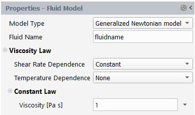
To specify a newtonian model, you need to first select .
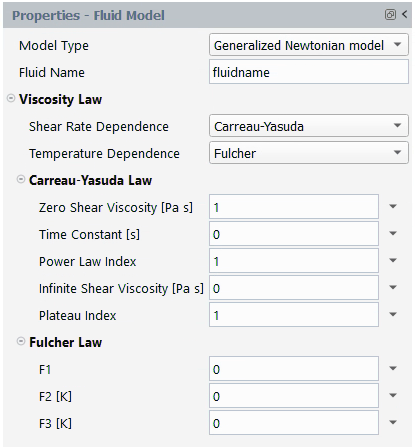
![]() Rheometry → Fluid
Model → Model Type
Rheometry → Fluid
Model → Model Type
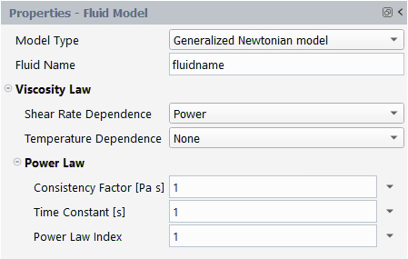
Specify an appropriate Fluid Name.
Choose the Shear Rate Dependence and Temperature Dependence law.
See Non-Automatic Fitting and Automatic Fitting for information about where and how the material data specification occurs in the non-automatic and automatic fitting procedures, respectively.
See Shear Rate Dependence of Viscosity and Temperature Dependence of Viscosity for details about the parameters and characteristics of each fluid model.
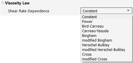
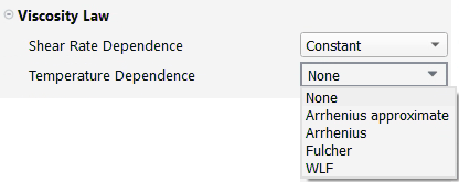
There are currently 10 laws available for  .
.
![]() Rheometry → Fluid
Model → Viscosity
Law → Shear Rate Dependence
Rheometry → Fluid
Model → Viscosity
Law → Shear Rate Dependence
![]() Rheometry → Fluid
Model → Viscosity
Law → Shear Rate
Dependence → Constant
Rheometry → Fluid
Model → Viscosity
Law → Shear Rate
Dependence → Constant
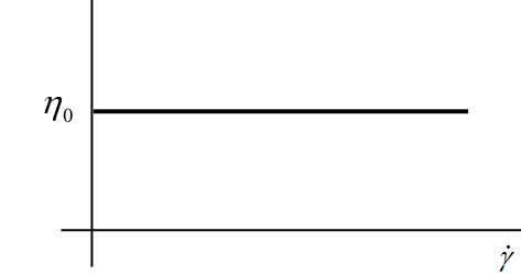
For Newtonian fluids, a constant viscosity
 | (4–30) |
is the default setting.  is referred to as the Newtonian or zero-shear-rate
viscosity, and its default value is 1.
is referred to as the Newtonian or zero-shear-rate
viscosity, and its default value is 1.
The units for  and its name in the Fluent Materials Processing interface are as
follows:
and its name in the Fluent Materials Processing interface are as
follows:
| Parameter | Name in MatPro Rheometry tool | Mass | Length | Time |
|---|---|---|---|---|
 | Viscosity [Pa s] | 1 | –1 | –1 |
Figure 4.125: Constant (Shear-Rate-Independent) Viscosity
shows a plot of a constant  .
.
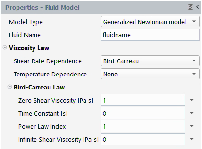
![]() Rheometry → Fluid
Model → Viscosity
Law → Shear Rate
Dependence → Bird-Carreau
Rheometry → Fluid
Model → Viscosity
Law → Shear Rate
Dependence → Bird-Carreau
The Bird-Carreau law for viscosity is
 | (4–31) |
where  is the infinite-shear-rate viscosity,
  is the zero-shear-rate viscosity,
  is natural time (that is, inverse of the shear rate at
which the fluid changes from Newtonian to power-law behavior) and
is natural time (that is, inverse of the shear rate at
which the fluid changes from Newtonian to power-law behavior) and
 is the power-law index.
The units for the parameters and their names in the Fluent Materials Processing interface are as follows:
| Parameter | Name in MatPro Rheometry tool | Mass | Length | Time |
|---|---|---|---|---|
 | Zero Shear Viscosity [Pa s] | 1 | –1 | –1 |
 | Infinite Shear Viscosity [Pa s] | 1 | –1 | –1 |
 | Time Constant [s] | 1 | ||
 | Power Law Index | – | – | – |
By default,  and
and  are equal to 1, and
  and
and  are equal to 0. Figure 4.126: Bird-Carreau Law for Viscosity shows a
plot of a
are equal to 0. Figure 4.126: Bird-Carreau Law for Viscosity shows a
plot of a  for the Bird-Carreau law.
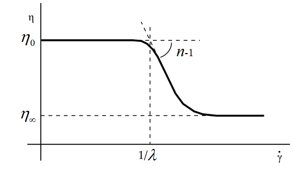
The Bird-Carreau law is commonly used when it is necessary to describe the low-shear-rate behavior of the viscosity. It differs from the Cross law primarily in the curvature of the viscosity curve in the vicinity of the transition between the plateau zone and the power law behavior.
![]() Rheometry → Fluid
Model → Viscosity
Law → Shear Rate
Dependence → Power
Rheometry → Fluid
Model → Viscosity
Law → Shear Rate
Dependence → Power
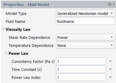
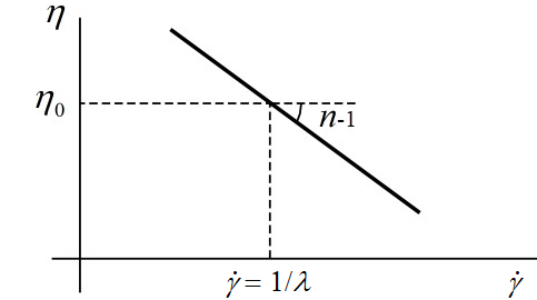
The power law for viscosity is
 | (4–32) |
where  is the consistency factor,
  is the natural time, and
  is the power-law index, which is a property of a given
material.
is the power-law index, which is a property of a given
material.
The units for the parameters and their names in the Fluent Materials Processing interface are as follows:
| Parameter | Name in MatPro Rheometry tool | Mass | Length | Time |
|---|---|---|---|---|
 | Consistency Factor [Pa s] | 1 | –1 | –1 |
 | Time Constant [s] | 1 | ||
 | Power Law Index | – | – | – |
By default,  ,
,  , and
, and  are equal to 1. Figure 4.127: Power Law for Viscosity shows a
plot of
are equal to 1. Figure 4.127: Power Law for Viscosity shows a
plot of  for the power law.
The power law is commonly used for the algebraic simplicity of its formulation. Although it can be a good candidate for describing the behavior of polyethylene or rubber for shear rates spanning over 2 or 3 decades, it does not predict any plateau for low shear rates. Consequently, it can be a convenient choice for the analysis of internal flow, but it should preferably be avoided when analyzing extrusion flows.
![]() Rheometry → Fluid
Model → Viscosity
Law → Shear Rate
Dependence → Bingham
Rheometry → Fluid
Model → Viscosity
Law → Shear Rate
Dependence → Bingham
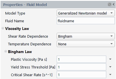
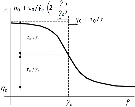
The Bingham law for viscosity is
 | (4–33) |
where  is the yield stress and
  is the critical shear rate, beyond which
Bingham’s constitutive equation is applied. For shear rates less
than
is the critical shear rate, beyond which
Bingham’s constitutive equation is applied. For shear rates less
than  , the behavior of the fluid is normalized in order to
mimic as much as possible a solid body and to guarantee appropriate
continuity properties in the viscosity curve.
, the behavior of the fluid is normalized in order to
mimic as much as possible a solid body and to guarantee appropriate
continuity properties in the viscosity curve.
The units for the parameters and their names in the Fluent Materials Processing interface are as follows:
| Parameter | Name in MatPro Rheometry tool | Mass | Length | Time |
|---|---|---|---|---|
 | Plastic Viscosity [Pa s] | 1 | –1 | –1 |
 | Yield Stress Threshold [Pa] | 1 | –1 | –2 |
 | Critical Shear Rate [s^-1] | – | – | –1 |
By default,  ,
,  , and
, and  are equal to 1. Figure 4.128: Bingham Law for Viscosity shows a plot
of
are equal to 1. Figure 4.128: Bingham Law for Viscosity shows a plot
of  for the Bingham law.
The Bingham law is commonly used to describe materials such as concrete, mud, dough, and toothpaste, for which a constant viscosity after a critical shear stress is a reasonable assumption, typically at rather low shear rates.
![]() Rheometry → Fluid
Model → Viscosity
Law → Shear Rate
Dependence → modified
Bingham
Rheometry → Fluid
Model → Viscosity
Law → Shear Rate
Dependence → modified
Bingham
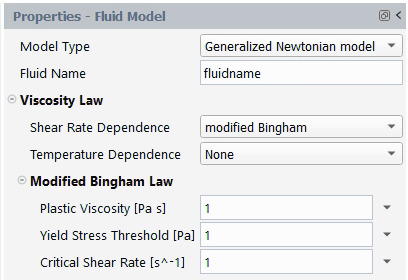
A modified Bingham law for viscosity is also available:
 | (4–34) |
where  .
.
The units for the parameters and their names in the Fluent Materials Processing interface are as follows:
| Parameter | Name in Rheometry Tool | Mass | Length | Time |
|---|---|---|---|---|
 | Plastic Viscosity [Pa s] | 1 | –1 | –1 |
 | Yield Stress Threshold [Pa] | 1 | –1 | –2 |
 | Critical Shear Rate [s^-1] | – | – | –1 |
By default,  ,
,  , and
, and  are equal to 1. Figure 4.129: Modified Bingham Law for Viscosity shows a
plot of
are equal to 1. Figure 4.129: Modified Bingham Law for Viscosity shows a
plot of  for the modified Bingham law.
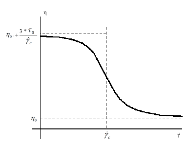
Compared to the standard Bingham law, the modified Bingham law is an
analytic expression, which means that it may be easier for
Fluent Materials Processing to calculate, leading to a more stable solution. The value
 has been selected so that the standard and modified
Bingham laws exhibit the same behavior above the critical shear rate,
has been selected so that the standard and modified
Bingham laws exhibit the same behavior above the critical shear rate,
 .
.
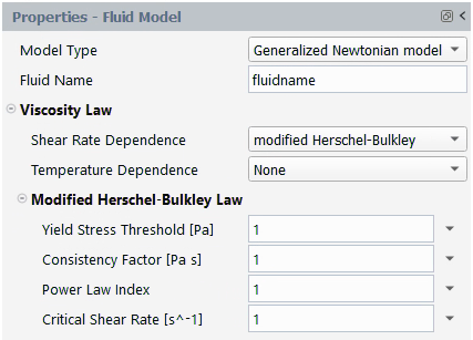
![]() Rheometry → Fluid
Model → Viscosity
Law → Shear Rate
Dependence → Herschel-Bulkley
Rheometry → Fluid
Model → Viscosity
Law → Shear Rate
Dependence → Herschel-Bulkley
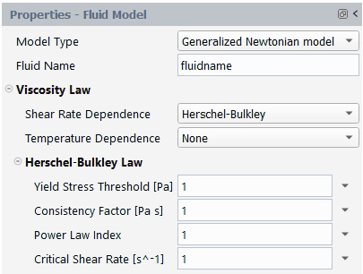
The Herschel-Bulkley law for viscosity is
 | (4–35) |
where  is the yield stress,
  is the critical shear rate,
  is the consistency factor, and
  is the power-law index.
The units for the parameters and their names in the Fluent Materials Processing interface are as follows:
| Parameter | Name in Rheometry Tool | Mass | Length | Time |
|---|---|---|---|---|
 | Yield Stress Threshold [Pa] | 1 | –1 | –2 |
 | Consistency Factor [Pa s] | 1 | –1 | –1 |
 | Critical Shear Rate [s^-1] | – | – | –1 |
 | Power Law Index | – | – | – |
By default,  ,
,  ,
,  , and
, and  are equal to 1. Figure 4.130: Herschel-Bulkley Law for Viscosity shows a plot of
  for the Herschel-Bulkley law.
Like the Bingham law, the Herschel-Bulkley law is commonly used to describe materials such as concrete, mud, dough, and toothpaste, for which a constant viscosity after a critical shear stress is a reasonable assumption. In addition to the transition behavior between a flow and no-flow regime, the Herschel-Bulkley law exhibits a shear-thinning behavior that the Bingham law does not.
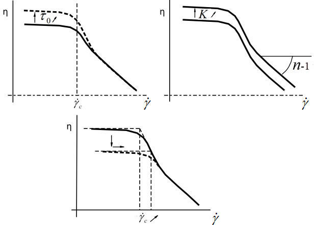
Note: An oblique arrow on the right of a symbol indicates how the symbol changes, and vertical/horizontal arrows indicate how the curve transforms as the symbol changes.
![]() Rheometry → Fluid
Model → Viscosity
Law → Shear Rate
Dependence → modified
Herschel-Bulkley
Rheometry → Fluid
Model → Viscosity
Law → Shear Rate
Dependence → modified
Herschel-Bulkley
A modified Herschel-Bulkley law is also available:
 | (4–36) |
The units for the parameters and their names in the Fluent Materials Processing interface are as follows:
| Parameter | Name in Rheometry Tool | Mass | Length | Time |
|---|---|---|---|---|
 | Yield Stress Threshold [Pa] | 1 | –1 | –2 |
 | Consistency Factor [Pa s] | 1 | –1 | –1 |
 | Critical Shear Rate [s^-1] | – | – | –1 |
 | Power Law Index | – | – | – |
By default,  ,
,  ,
,  , and
, and  are equal to 1. Figure 4.131: Modified Herschel-Bulkley Law for Viscosity shows a plot
of
are equal to 1. Figure 4.131: Modified Herschel-Bulkley Law for Viscosity shows a plot
of  for the modified Herschel-Bulkley law.
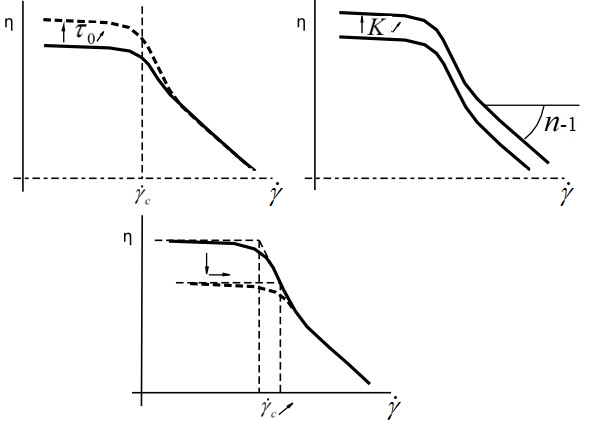
Compared to the standard Herschel-Bulkley law, Figure 4.130: Herschel-Bulkley Law for Viscosity, the modified Herschel-Bulkley law is
an analytic expression, which means that it may be easier for
Fluent Materials Processing to calculate, leading to a more stable solution. The
integer value 3 that appears in the argument of the
exponential term has been selected so that the standard and modified
Herschel-Bulkley laws exhibit the same behavior above the critical shear
rate,  .
.
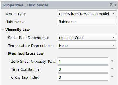
![]() Rheometry → Fluid
Model → Viscosity
Law → Shear Rate
Dependence → Cross
Rheometry → Fluid
Model → Viscosity
Law → Shear Rate
Dependence → Cross
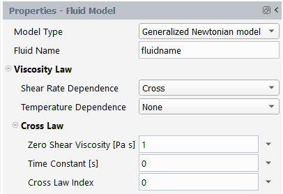
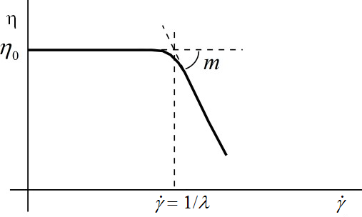
The Cross law for viscosity is
 | (4–37) |
where  is the zero-shear-rate viscosity,
  is the natural time (that is, inverse of the shear
rate at which the fluid changes from Newtonian to power-law behavior)
and
is the natural time (that is, inverse of the shear
rate at which the fluid changes from Newtonian to power-law behavior)
and  is the Cross-law index (= 1–
 for large shear rates).
The units for the parameters and their names in the Fluent Materials Processing interface are as follows:
| Parameter | Name in Fluent Materials Processing | Mass | Length | Time |
|---|---|---|---|---|
 | Zero Shear Viscosity [Pa s] | 1 | 1 | –1 |
 | Time Constant [s] | 1 | ||
 | Cross Law Index | – | – | – |
By default,  is equal to 1, and
  and
and  are equal to 0. Figure 4.132: Cross Law for Viscosity shows a plot of
 for the Cross law.
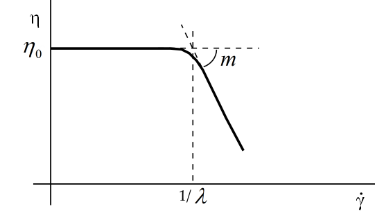
Like the Bird-Carreau law, the Cross law is commonly used when it is necessary to describe the low-shear-rate behavior of the viscosity. It differs from the Bird-Carreau law primarily in the curvature of the viscosity curve in the vicinity of the transition between the plateau zone and the power law behavior.
![]() Rheometry → Fluid
Model → Viscosity
Law → Shear Rate
Dependence → modified
Cross
Rheometry → Fluid
Model → Viscosity
Law → Shear Rate
Dependence → modified
Cross
A modified Cross law for viscosity is also available:
 | (4–38) |
The units for the parameters and their names in the Fluent Materials Processing interface are as follows:
| Parameter | Name in Fluent Materials Processing | Mass | Length | Time |
|---|---|---|---|---|
 | Zero Shear Viscosity [Pa s] | 1 | 1 | –1 |
 | Time Constant [s] | 1 | ||
 | Cross Law Index | – | – | – |
By default,  is equal to 1, and
  and
and  are equal to 0. Figure 4.133: Modified Cross Law for Viscosity shows a
plot of
are equal to 0. Figure 4.133: Modified Cross Law for Viscosity shows a
plot of  for the Cross law.
This law can be considered a special case of the Carreau-Yasuda
viscosity law (Equation 4–39), where the exponent  has a value of 1.
![]() Rheometry → Fluid
Model → Viscosity
Law → Shear Rate
Dependence → Carreau-Yasuda
Rheometry → Fluid
Model → Viscosity
Law → Shear Rate
Dependence → Carreau-Yasuda
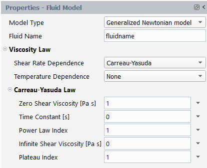
The Carreau-Yasuda law for viscosity is:
 | (4–39) |
where  is the zero-shear-rate viscosity,
  is the infinite-shear-rate viscosity,
  is the natural time (that is, inverse of the shear
rate at which the fluid changes from Newtonian to power-law behavior),
is the natural time (that is, inverse of the shear
rate at which the fluid changes from Newtonian to power-law behavior),
 is the index that controls the transition from the
Newtonian plateau to the power-law region and
is the index that controls the transition from the
Newtonian plateau to the power-law region and  is the power-law index.
The units for the parameters and their names in the Fluent Materials Processing interface are as follows:
| Parameter | Name in Fluent Materials Processing | Mass | Length | Time |
|---|---|---|---|---|
 | Zero Shear Viscosity [Pa s] | 1 | –1 | –1 |
 | Infinite Shear Viscosity [Pa s] | 1 | –1 | –1 |
 | Time Constant [s] | 1 | ||
 | Power Law Index | – | – | – |
 | Plateau Index | – | – | – |
By default,  ,
,  , and
, and  are equal to 1, and
  and
and  are equal to 0. Figure 4.134: Carreau-Yasuda Law for Viscosity shows
a plot of
are equal to 0. Figure 4.134: Carreau-Yasuda Law for Viscosity shows
a plot of  for the Carreau-Yasuda law.
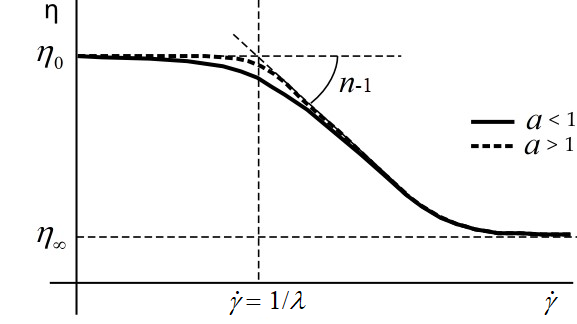
The Carreau-Yasuda law is a slight variation on the Bird-Carreau law
(Equation 4–31).
The addition of the exponent  allows for control of the transition from the
Newtonian plateau to the power-law region. A low value (
allows for control of the transition from the
Newtonian plateau to the power-law region. A low value ( < 1) lengthens the transition, and a high value
(
< 1) lengthens the transition, and a high value
( >1) results in an abrupt transition.
![]() Rheometry → Fluid
Model → Viscosity
Law → Temperature Dependence
Rheometry → Fluid
Model → Viscosity
Law → Temperature Dependence
As discussed in Introduction, the general form for the viscosity  can be written as the product of functions of shear rate
and temperature. There are two ways in which this relationship can be
expressed:
can be written as the product of functions of shear rate
and temperature. There are two ways in which this relationship can be
expressed:
 | (4–40) |
 | (4–41) |
where  and
and  represent the shear-rate and temperature dependence of the
viscosity, respectively.
represent the shear-rate and temperature dependence of the
viscosity, respectively.
In Equation 4–40, the
temperature scales the viscosity so there is only a vertical shift on the
model curves  vs. temperature. Four of the temperature-dependent
laws follow this format:
vs. temperature. Four of the temperature-dependent
laws follow this format:
Arrhenius approximate law
Arrhenius law
Fulcher law
WLF law
In Equation 4–41, the
time-temperature equivalence is introduced by also scaling the shear rate by
temperature. Therefore, there is a horizontal shift in addition to the
vertical shift on the model curves  vs. temperature. Three of the temperature-dependent
viscosity laws follow this format:
vs. temperature. Three of the temperature-dependent
viscosity laws follow this format:
Arrhenius approximate law
Arrhenius law
WLF law
By default, there is no temperature dependence of the viscosity (that is,
 ).
).
![]() Rheometry → Fluid
Model → Viscosity
Law → Temperature
Dependence → Arrhenius
Rheometry → Fluid
Model → Viscosity
Law → Temperature
Dependence → Arrhenius
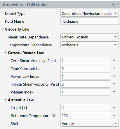
The Arrhenius law is given as
 | (4–42) |
where  is the ratio of the activation energy to the perfect
gas constant and
is the ratio of the activation energy to the perfect
gas constant and  is a reference temperature for which
  .
.
The units for the parameters and their names in the Fluent Materials Processing interface are as follows:
| Parameter | Name in MatPro Rheometry Tool | Mass | Length | Time | Temperature |
|---|---|---|---|---|---|
 | Ea/R [K] | – | – | – | 1 |
 | Reference Temperature [K] | – | – | – | 1 |
By default, Ea/R is set to 0 and the
Reference Temperature to 300 [K]. Figure 4.135: Arrhenius Law for the Temperature Dependence of the Viscosity
With Vertical Shift Only shows a plot of
 for the Arrhenius law.
Figure 4.135: Arrhenius Law for the Temperature Dependence of the Viscosity With Vertical Shift Only
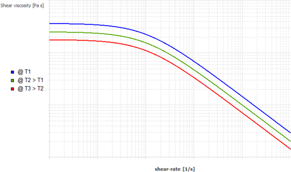
When the Arrhenius law is selected for the temperature dependence of the viscosity, you have the option of selecting the shift that is applied such as a vertical shift only or a combination of both vertical and horizontal shifts. If the vertical shift is selected, the viscosity curve will be shifted vertically, downwards or upwards, subsequently to a temperature increase or decrease, respectively. Figure 4.135: Arrhenius Law for the Temperature Dependence of the Viscosity With Vertical Shift Only suggests a vertical shift only, where Equation 4–40 is used. Figure 4.136: Approximate Arrhenius Law for the Temperature Dependence of the Viscosity With Both Vertical and Horizontal Shifts suggests a combination of both vertical and horizontal shifts, where Equation 4–41 is applied.
![]() Rheometry → Fluid
Model → Viscosity
Law → Temperature
Dependence → Arrhenius
approximate
Rheometry → Fluid
Model → Viscosity
Law → Temperature
Dependence → Arrhenius
approximate
The approximate Arrhenius law is obtained as the first-order Taylor expansion of the Arrhenius law (Equation 4–42):
 | (4–43) |
Where  is the ratio of the activation energy to the perfect
gas constant and
is the ratio of the activation energy to the perfect
gas constant and  is a reference temperature for which H(T) = 1. The
behavior described by Equation 4–43 is similar to that described by Equation 4–42 in the
neighborhood of
is a reference temperature for which H(T) = 1. The
behavior described by Equation 4–43 is similar to that described by Equation 4–42 in the
neighborhood of  . Equation 4–43 is valid as long as the temperature difference
 is not too large.
The units for the parameters and their names in the Fluent Materials Processing interface are as follows:
| Parameter | Name in MatPro Rheometry Tool | Mass | Length | Time | Temperature |
|---|---|---|---|---|---|
 | Ea/R [K] | – | – | – | 1 |
 | Reference Temperature [K] | – | – | – | 1 |
By default, Ea/R is set to 0 and the
Reference Temperature is set to 300 [K]. Figure 4.136: Approximate Arrhenius Law for the Temperature Dependence of the
Viscosity With Both Vertical and Horizontal Shifts shows a
plot of  (
( ) for the approximate Arrhenius law.
Figure 4.136: Approximate Arrhenius Law for the Temperature Dependence of the Viscosity With Both Vertical and Horizontal Shifts
When the approximate Arrhenius law is selected for the temperature dependence of the viscosity, you have the option of selecting the shift that is applied such as a vertical shift only or a combination of both vertical and horizontal shifts. If the vertical shift is selected, the viscosity curve will be shifted vertically, downwards or upwards, subsequently to a temperature increase or decrease, respectively. Figure 4.135: Arrhenius Law for the Temperature Dependence of the Viscosity With Vertical Shift Only suggests a vertical shift only, where equation (Equation 4–40) is used. Figure 4.136: Approximate Arrhenius Law for the Temperature Dependence of the Viscosity With Both Vertical and Horizontal Shifts suggests a combination of both vertical and horizontal shifts, where equation (Equation 4–41) is applied.
![]() Rheometry → Fluid
Model → Viscosity
Law → Temperature
Dependence → Fulcher
Rheometry → Fluid
Model → Viscosity
Law → Temperature
Dependence → Fulcher
Another definition for  comes from the Fulcher law 5:
 | (4–44) |
where  ,
,  , and
, and  are the Fulcher constants. The Fulcher law is used
mainly for glass.
are the Fulcher constants. The Fulcher law is used
mainly for glass.
The units for the parameters and their names in the Fluent Materials Processing interface are as follows:
| Parameter | Name in MatPro Rheometry Tool | Mass | Length | Time | Temperature |
|---|---|---|---|---|---|
 | F1 | – | – | – | – |
 | F2 [K] | – | – | – | 1 |
 | F3 [K] | – | – | – | 1 |
By default,  ,
,  and
and  are equal to 0.
Although the Fulcher temperature dependence law can be combined with a
non-constant shear-rate dependence, it is originally developed for
modelling the temperature dependence of the viscosity for molten glass.
Hence, it is usually combined with a constant (unity) viscosity factor.
You can give the following interpretation for the three coefficients
 ,
,  and
and  .
.
As illustrated in Figure 4.137: Typical Viscosity Curve vs. Temperature, very high
temperature are encountered. You start with  , which corresponds to the temperature where the
viscosity is infinite. The law can no longer be applied if the fluid
temperature is lower than
, which corresponds to the temperature where the
viscosity is infinite. The law can no longer be applied if the fluid
temperature is lower than  . For preventing issues, a cut-off has been introduced
so that the calculation is not hindered when temperatures less than
. For preventing issues, a cut-off has been introduced
so that the calculation is not hindered when temperatures less than
 are encountered.
If  increases, the overall viscosity curve decreases.
Eventually, an increase of
increases, the overall viscosity curve decreases.
Eventually, an increase of  leads to a more visible dependence of the viscosity
curve with respect to the temperature.
leads to a more visible dependence of the viscosity
curve with respect to the temperature.
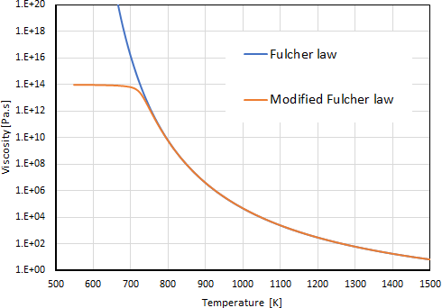
In the image above, the blue line is obeying the Fulcher Law and the viscosity can be bounded to prevent numerical issues (orange line).
In Figure 4.137: Typical Viscosity Curve vs. Temperature, you
plot the Fulcher viscosity curve vs. temperature. Very high values are
obtained at low temperatures. The law as such does not permit
considering temperatures below the value of . To prevent numerical difficulties which may originate
from very high values, an upper bound of 1014
has been assigned to the viscosity by default. That value is sufficient
for mimicking the behavior of a body which is partly solidified.
![]() Rheometry → Fluid
Model → Viscosity
Law → Temperature
Dependence → WLF
Rheometry → Fluid
Model → Viscosity
Law → Temperature
Dependence → WLF
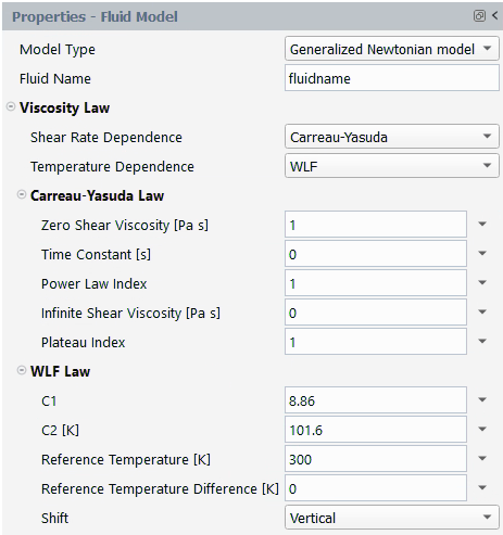
The Williams-Landel-Ferry (WLF) equation is a temperature-dependent viscosity law that fits experimental data better than the Arrhenius law for a wide range of temperatures, especially close to the glass transition temperature:
 | (4–45) |
where  and
and  are the WLF constants, and
  and
and  are reference temperatures.
The units for the parameters and their names in the Fluent Materials Processing interface are as follows:
| Parameter | Name in MatPro Rheometry Tool | Mass | Length | Time | Temperature |
|---|---|---|---|---|---|
 | C1 | – | – | – | – |
 | C2 [K] | – | – | – | 1 |
 | Reference Temperature [K] | – | – | – | 1 |
 | Reference Temperature Difference [K] | – | – | – | 1 |
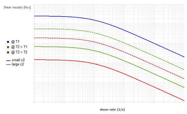
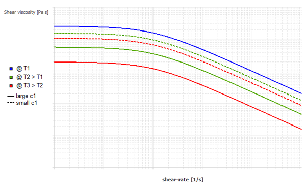
Figure 4.138: Effect of Increasing c2 on the WLF Law for Viscosity and
Figure 4.139: Effect of Increasing c1 or Ta on the WLF Law for
Viscosity show the
impact of each parameter on the viscosity curves. A large value of
 will enhance the decrease of the viscosity with
respect to temperature, while a larger value of
will enhance the decrease of the viscosity with
respect to temperature, while a larger value of  will spread out the viscosity dependence with respect
to temperature when it is around the reference temperature value.
will spread out the viscosity dependence with respect
to temperature when it is around the reference temperature value.
It is important to note that the quantity  must remain positive in a flow simulation.
When the WLF law is selected for the temperature dependence of the viscosity, you have the option of selecting the shift that is applied such as a vertical shift only or a combination of both vertical and horizontal shifts. If the vertical shift is selected, the viscosity curve will be shifted vertically, downwards, or upwards, subsequently to a temperature increase or decrease, respectively. Figure 4.136: Approximate Arrhenius Law for the Temperature Dependence of the Viscosity With Both Vertical and Horizontal Shifts suggests a vertical shift only, where equation (Equation 4–40) is used.
This section describes the following topics:
The differential approach to modeling viscoelastic model is appropriate for most practical applications. Many of the most common constitutive models for viscoelastic model are provided in Fluent Materials Processing, including Maxwell, Oldroyd, Phan-Thien-Tanner, Giesekus, FENE-P, POM-POM, and Leonov models. Appropriate choices for the viscoelastic model and related parameters can yield qualitatively and quantitatively accurate representations of viscoelastic behavior.
Improved accuracy is possible if you use multiple relaxation times to better fit the viscoelastic behavior at different shear rates.
Note: While differential viscoelastic models are compatible with 2D and 3D models, they are not compatible with the shell model.
For a differential viscoelastic model, the constitutive equation for the extra-stress tensor is
 | (4–46) |
 (the viscoelastic component) is computed differently
for each type of viscoelastic model.
(the viscoelastic component) is computed differently
for each type of viscoelastic model.  (the purely viscous component) is an optional
component, which is always computed from
(the purely viscous component) is an optional
component, which is always computed from
 | (4–47) |
where  is the rate-of-deformation tensor and
  is the viscosity factor for the Newtonian (that is,
purely viscous) component of the extra-stress-tensor referred to as the
additional viscosity.
is the viscosity factor for the Newtonian (that is,
purely viscous) component of the extra-stress-tensor referred to as the
additional viscosity.
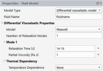
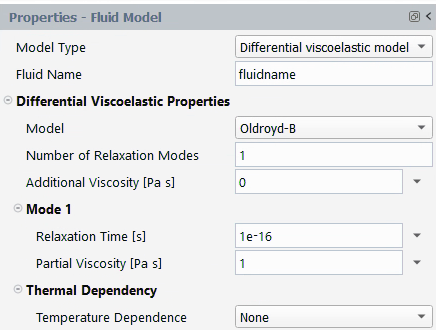
To specify a viscoelastic model, you need to first select Differential Viscoelastic model.
![]() Rheometry → Fluid
Model → Model Type
Rheometry → Fluid
Model → Model Type
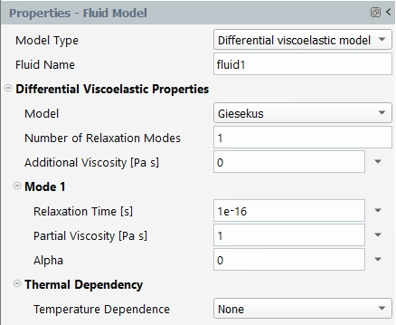
Specify an appropriate Fluid Name.
Choose the Model and specify Number of Relaxation Modes and Additional Viscosity [Pa s].
For each Mode, specify Relaxation Time [s], Partial Viscosity [Pa s] and Alpha.
Finally, select the law and parameters for the Thermal Dependency.
See Non-Automatic Fitting and Automatic Fitting for information about where and how the material data specification occurs in the non-automatic and automatic fitting procedures, respectively.
See Differential Viscoelastic Models and Temperature Dependence of Viscosity and Relaxation Time for details about the parameters and characteristics of each fluid model.
![]() Rheometry → Fluid
Model → Differential Viscoelastic
Properties → Model
Rheometry → Fluid
Model → Differential Viscoelastic
Properties → Model
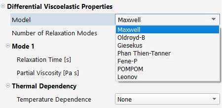
There are currently eight differential models:
and :
These are the simplest viscoelastic constitutive equations, although in many situations they are the most numerically cumbersome. Both models exhibit a constant viscosity and a quadratic first normal-stress difference. They should be selected either when very little information is known about the fluid, or when a qualitative prediction is sufficient. For fluids exhibiting a very high extensional viscosity, the model is preferred over the Maxwell model.
, Johnson-Segalman, and :
These models are the most realistic. They exhibit shear thinning and a non-quadratic first normal-stress difference at high shear rates. These properties are controlled by their respective material parameters (
 ,
,  , and
, and  ), as described in the model description below.
Also, the selection of nonzero values for
), as described in the model description below.
Also, the selection of nonzero values for  and
and  will lead to a bounded steady extensional
viscosity.
will lead to a bounded steady extensional
viscosity. For stability reasons in a simple shear flow, a non-zero additional viscosity must be selected. This is true for the Johnson-Segalman and models when
 is nonzero, and for the
model when
is nonzero, and for the
model when  >0.5. The addition of a purely viscous component
to the extra-stress tensor affects the viscosity, but not the first
normal-stress difference. Shear thinning is still present, but the
viscosity curve also shows a plateau zone at high shear rates.
>0.5. The addition of a purely viscous component
to the extra-stress tensor affects the viscosity, but not the first
normal-stress difference. Shear thinning is still present, but the
viscosity curve also shows a plateau zone at high shear rates. Poor control of the shear viscosity is the usual drawback of the Johnson-Segalman and models used with a single relaxation time, especially toward high shear rates.
Important: Note that you cannot explicitly select the Johnson-Segalman model in the Fluent Materials Processing interface. It is obtained by selecting the model and setting the value of
 to 0.
to 0.:
A single mode of the model requires only three parameters (
 ,
,  and the length ratio for the spring), yet it
predicts a realistic shear thinning of the fluid and a first
normal-stress difference that is quadratic for low shear rates and
has a lower slope for high shear rates. It has been observed in
practice that viscometric properties of several fluids can often be
accurately modeled. The model is well
suited for simulating the rheological behavior of dilute
solutions.
and the length ratio for the spring), yet it
predicts a realistic shear thinning of the fluid and a first
normal-stress difference that is quadratic for low shear rates and
has a lower slope for high shear rates. It has been observed in
practice that viscometric properties of several fluids can often be
accurately modeled. The model is well
suited for simulating the rheological behavior of dilute
solutions.:
The pom-pom molecule consists of a backbone to which
 arms are connected at both extremities. In a flow,
the backbone may orient in a Doi-Edwards reptation tube consisting
of the neighboring molecules, while the arms may retract into that
tube. The concept of the pom-pom macromolecule makes the model
suitable for describing the behavior of branched polymers. The
approximate differential form of the model is based on the equations
of macromolecular orientation and macromolecular stretching in
connection with changes in orientation. In this construction, the
pom-pom molecule is allowed only a finite extension, which is
controlled by the number of dangling arms. In particular, the strain
hardening properties are dictated by the number of arms. Beyond
that, the model predicts realistic shear thinning behavior, as well
as a first and a possible second normal stress difference.
arms are connected at both extremities. In a flow,
the backbone may orient in a Doi-Edwards reptation tube consisting
of the neighboring molecules, while the arms may retract into that
tube. The concept of the pom-pom macromolecule makes the model
suitable for describing the behavior of branched polymers. The
approximate differential form of the model is based on the equations
of macromolecular orientation and macromolecular stretching in
connection with changes in orientation. In this construction, the
pom-pom molecule is allowed only a finite extension, which is
controlled by the number of dangling arms. In particular, the strain
hardening properties are dictated by the number of arms. Beyond
that, the model predicts realistic shear thinning behavior, as well
as a first and a possible second normal stress difference.:
This model has been developed for the simultaneous prediction of the behavior of trapped and free macromolecular chains for filled elastomers with carbon black and/or silicate. From the point of view of morphology, macromolecules at rest are trapped by particles of carbon black, via electrostatic van der Waals forces. Under a deformation field, electrostatic bonds can break, and macromolecules become free, while a reverse mechanism may develop when the deformation ceases. You can therefore be facing a macromolecular system consisting of trapped and free macromolecules, with a reversible transition from one state to the other one.
This model involves two tensor quantities and a scalar one. The tensors focus respectively on the behavior of the free and trapped macromolecular chains of the elastomer, while the scalar variable quantifies the degree of structural damage (debonding factor). The model exhibits a yielding behavior. It is intrinsically nonlinear, as the nonlinear response develops and is observable at early deformations.
Details about each model are provided below.
![]() Rheometry → Fluid
Model → Differential Viscoelastic
Properties → Model →
Maxwell
Rheometry → Fluid
Model → Differential Viscoelastic
Properties → Model →
Maxwell
The Maxwell model is one of the simplest viscoelastic constitutive equations. It exhibits a constant viscosity and a quadratic first normal-stress difference. Due to its simplicity, it is recommended only when little information about the fluid is available, or when a qualitative prediction is sufficient. Even in this case, the Oldroyd-B model, which can include a purely viscous component, is preferable for numerical reasons.
The equation for the Maxwell model is the upper-convected Maxwell
model, in which the purely viscous component of the extra-stress
tensor ( ) is equal to zero. For single-mode, the
viscoelastic component (
) is equal to zero. For single-mode, the
viscoelastic component ( ) is computed from
 | (4–48) |
where  is a model-specific relaxation time,
 is the rate-of-deformation tensor, and
 is a model-specific viscosity factor for the
viscoelastic component of
is a model-specific viscosity factor for the
viscoelastic component of  . The relaxation time
  is defined as the time required for the shear
stress to be reduced to half of its original equilibrium value when
the strain rate vanishes. A high relaxation time indicates that the
memory retention of the flow is high. A low relaxation time
indicates significant memory loss, gradually approaching Newtonian
flow (zero relaxation time).
is defined as the time required for the shear
stress to be reduced to half of its original equilibrium value when
the strain rate vanishes. A high relaxation time indicates that the
memory retention of the flow is high. A low relaxation time
indicates significant memory loss, gradually approaching Newtonian
flow (zero relaxation time).
The units for the parameters and their names in the Fluent Materials Processing interface are as follows:
| Parameter | Name in Fluent Materials Processing | Mass | Length | Time |
|---|---|---|---|---|
 | Partial Viscosity [Pa s] | 1 | –1 | –1 |
 | Relaxation Time [s] | – | – | 1 |
By default, is set to 1 and  to 10-16.
Additionally, by default, Number of Relaxation
Modes is set to 1. You can select multiple relaxation
modes, in which case multiple sets of parameters will have to be
specified ( ,
,  ).
).
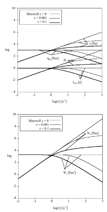
Figure 4.140: Maxwell Model for a Shear Flow shows the viscometric functions of the Maxwell
model in a simple shear flow. In this example (where  =1 s and
  =1000 Pa-s),
  is constant,
  is linear,
  is quadratic,
  is zero,
  is constant,
  is zero, and
  is linear, showing non-asymptotic behavior.
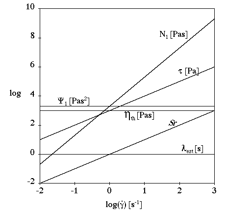
Figure 4.141: Maxwell Model for an Extensional Flow shows the behavior of the Maxwell model in a simple extensional flow.
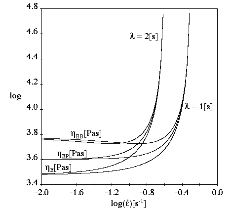
In this example (where  =1 s and
  =1000 Pa-s),
  ,
,  , and
, and  are unbounded for
  , and
, and
 | (4–49) |
 | (4–50) |
 | (4–51) |
 | (4–52) |
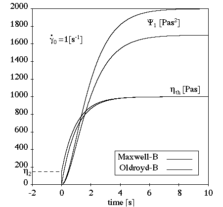
Figure 4.142: Maxwell Model for a Transient Shear Flow shows the behavior of the Maxwell model in a transient shear flow.
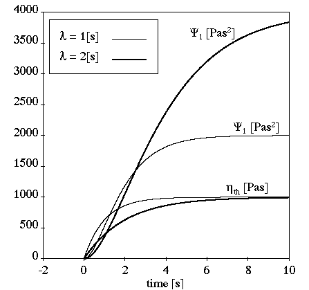
In this example (where  =1 s,
=1 s,  =1000 Pa-s, and
  s-1), there is no
stress overshoot and the transient phase depends upon the relaxation
time.
s-1), there is no
stress overshoot and the transient phase depends upon the relaxation
time.
![]() Rheometry → Fluid
Model → Differential Viscoelastic
Properties → Model →
Oldroyd-B
Rheometry → Fluid
Model → Differential Viscoelastic
Properties → Model →
Oldroyd-B
The Oldroyd-B model, like the Maxwell model, is one of the simplest viscoelastic constitutive equations. It is slightly better than the Maxwell model, because it allows for the inclusion of the purely viscous component of the extra stress, which leads to better behavior of the numerical scheme. Oldroyd-B is a good choice for fluids that exhibit a very high extensional viscosity.
For the Oldroyd-B model,  is computed from Equation 4–48, and
  is computed (optionally) from Equation 4–47.
  from Equation 4–48 is the partial
viscosity, while
from Equation 4–48 is the partial
viscosity, while  in Equation 4–47 is the additional viscosity
The units for the parameters and their names in the Fluent Materials Processing interface are as follows:
| Parameter | Name in Fluent Materials Processing | Mass | Length | Time |
|---|---|---|---|---|
| | Partial Viscosity [Pa s] | 1 | –1 | –1 |
 | Relaxation Time [s] | – | – | 1 |
| | Additional Viscosity [Pa s] | 1 | –1 | –1 |
By default, is set to 1 while is set to 10-16.
 is set to 0.
Additionally, by default, Number of Relaxation
Modes is set to 1. You can select multiple relaxation
modes, in which case multiple sets of parameters will have to be
specified (, ).
Figure 4.143: Oldroyd-B Model for a Shear Flow shows the viscometric functions of the
Oldroyd-B model in a simple shear flow. In this example,
 =1 s and (with the viscosity ratio equal to 0.15)
 =850 Pa-s and
  =150 Pa-s. In the resulting curves,
 is constant,
  is linear,
  is quadratic,
  is zero,
  is constant,
  is zero, and
  is linear, showing non-asymptotic behavior. Notice
that the curves are moved down in comparison to the Maxwell model;
this is due to the Newtonian part of the model (nonzero value for
is linear, showing non-asymptotic behavior. Notice
that the curves are moved down in comparison to the Maxwell model;
this is due to the Newtonian part of the model (nonzero value for
 ), which reduces the viscoelastic effects
(
), which reduces the viscoelastic effects
( ,
,  ,
,  , and
, and  ).
).
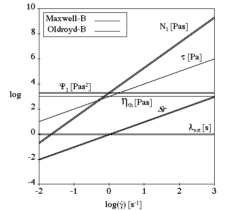
Figure 4.144: Oldroyd-B Model for a Transient Shear Flow shows the behavior of the Oldroyd-B model in a
transient shear flow. In this example,  =1 s,
=1 s,  =1000 Pa-s, and
  s–1. Notice
that there is an instantaneous response of the shear stress to the
applied shear rate; this is due to the Newtonian part of the model
originating from the additional viscosity whose value was set to 150
Pa.s. Otherwise, the Oldroyd-B model exhibits the same behavior as
the Maxwell model.
s–1. Notice
that there is an instantaneous response of the shear stress to the
applied shear rate; this is due to the Newtonian part of the model
originating from the additional viscosity whose value was set to 150
Pa.s. Otherwise, the Oldroyd-B model exhibits the same behavior as
the Maxwell model.
![]() Rheometry → Fluid
Model → Differential Viscoelastic
Properties → Model →
Phan-Thien-Tanner
Rheometry → Fluid
Model → Differential Viscoelastic
Properties → Model →
Phan-Thien-Tanner
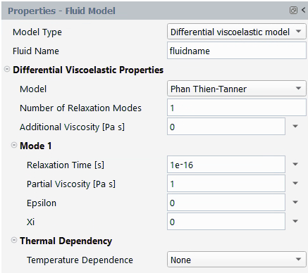
The Phan-Thien-Tanner model is one of the most realistic differential viscoelastic models. It exhibits shear thinning and a non-quadratic first normal-stress difference at high shear rates.
The PTT model computes  from
from
 | (4–53) |
and  is computed (optionally) from Equation 4–47. in Equation 4–53 is the partial viscosity, while in Equation 4–47 is the additional viscosity.
 and
and  are material properties that control,
respectively, the shear viscosity and elongational behavior. A
nonzero value for
are material properties that control,
respectively, the shear viscosity and elongational behavior. A
nonzero value for  leads to a bounded steady extensional
viscosity.
leads to a bounded steady extensional
viscosity.
The units for the parameters and their names in the Fluent Materials Processing interface are as follows:
| Parameter | Name in Fluent Materials Processing | Mass | Length | Time |
|---|---|---|---|---|
 | Partial Viscosity [Pa s] | 1 | –1 | –1 |
 | Relaxation Time [s] | – | – | 1 |
 | Additional Viscosity [Pa s] | 1 | –1 | –1 |
 | Epsilon | – | – | – |
 | Xi | – | – | – |
By default,  is set to 1 while
  is set to 10-16.
 is set to 0.
  and
and  are also set to 0 by default.
Additionally, by default, Number of Relaxation
Modes is set to 1. You can select multiple relaxation
modes, in which case multiple sets of parameters will have to be
specified (, ,  ,
,  ).
).
In a simple shear flow (Figure 4.145: PTT Model for a Shear Flow), for  >0, you can see a shear-thinning effect and a
non-quadratic behavior for the first normal-stress difference
>0, you can see a shear-thinning effect and a
non-quadratic behavior for the first normal-stress difference
 . You will also notice that, for
  >0, the elasticity level
  remains finite for increasing shear rate
(asymptotic behavior).
remains finite for increasing shear rate
(asymptotic behavior).
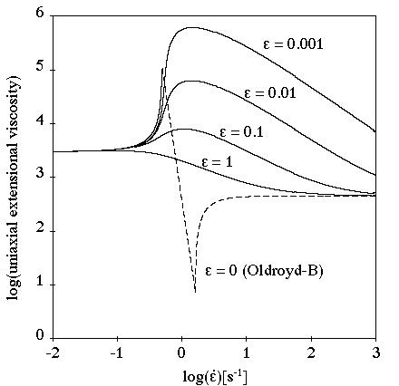
The parameter  also affects the extensional viscosities, as shown
in Figure 4.146: PTT Model for a Steady Extensional Flow. The steady extensional viscosities are finite,
and tend toward the Newtonian component of the extensional viscosity
(that is, they are uniaxial) for large extension rates. For small
values of
also affects the extensional viscosities, as shown
in Figure 4.146: PTT Model for a Steady Extensional Flow. The steady extensional viscosities are finite,
and tend toward the Newtonian component of the extensional viscosity
(that is, they are uniaxial) for large extension rates. For small
values of  , there is extension thickening and thinning; for
large values, there is only extension thinning.
, there is extension thickening and thinning; for
large values, there is only extension thinning.
Important: For a single-mode PTT model, if the parameter  is not zero, then the additional viscosity
must be at least 1/8 of the Partial
Viscosity in order to ensure the stability of the
shear flow. However, this value may decrease when
is not zero, then the additional viscosity
must be at least 1/8 of the Partial
Viscosity in order to ensure the stability of the
shear flow. However, this value may decrease when
 does not vanish. The slope of the shear stress
vs. shear rate curve must be positive everywhere, contrary to
what is shown on the left in Figure 4.147: Effect of ξ on the PTT Model for a Shear Flow with
does not vanish. The slope of the shear stress
vs. shear rate curve must be positive everywhere, contrary to
what is shown on the left in Figure 4.147: Effect of ξ on the PTT Model for a Shear Flow with  =0.1.
=0.1.
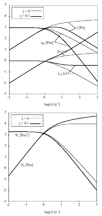
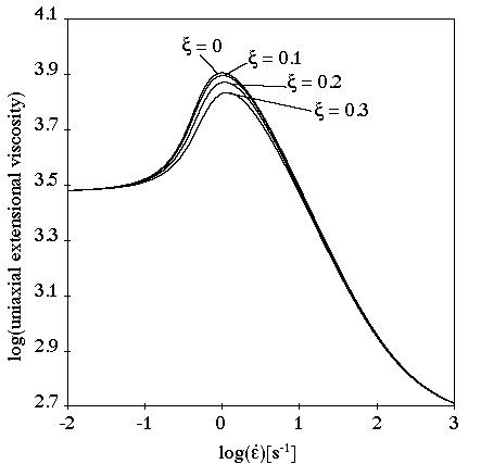
The parameter  has almost no effect on extensional viscosity, as
shown in Figure 4.148: Effect of ξ on the PTT Model for a Steady Extensional
Flow. The maximum of the extensional viscosities
decreases when
has almost no effect on extensional viscosity, as
shown in Figure 4.148: Effect of ξ on the PTT Model for a Steady Extensional
Flow. The maximum of the extensional viscosities
decreases when  increases.
In a transient shear flow (Figure 4.149: PTT Model in a Transient Shear Flow), a moderate stress overshoot is observed. The stress overshoot increases as shear rate increases. Shear thinning is observed, and the normal stress is non-quadratic. The transient phase is reduced as the shear rate increases.
![]() Rheometry → Fluid
Model → Differential Viscoelastic
Properties → Model →
Giesekus
Rheometry → Fluid
Model → Differential Viscoelastic
Properties → Model →
Giesekus
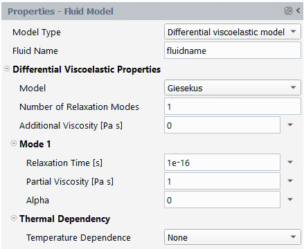
Like the PTT model, the Giesekus model is one of the most realistic differential viscoelastic models. It exhibits shear thinning and a non-quadratic first normal-stress difference at high shear rates.
The Giesekus model computes  from
from
 | (4–54) |
and  is computed (optionally) from Equation 4–47. in Equation 4–54 is the partial
viscosity, while in Equation 4–47 is the additional viscosity.
is computed (optionally) from Equation 4–47. in Equation 4–54 is the partial
viscosity, while in Equation 4–47 is the additional viscosity.
 is the unit tensor and
  is a material constant that controls the
extensional viscosity and the ratio of the second normal-stress
difference to the first. For low values of shear rate,
is a material constant that controls the
extensional viscosity and the ratio of the second normal-stress
difference to the first. For low values of shear rate,
 | (4–55) |
For the majority of fluids, this ratio is between 0.1 and 0.2.
The units for the parameters and their names in the Fluent Materials Processing interface are as follows:
| Parameter | Name in Fluent Materials Processing | Mass | Length | Time |
|---|---|---|---|---|
 | Partial Viscosity [Pa s] | 1 | –1 | –1 |
 | Relaxation Time [s] | – | – | 1 |
 | Additional Viscosity [Pa s] | 1 | –1 | –1 |
 | Alpha | – | – | – |
By default,  is set to 1 while
  is set to 10-16.
 is set to 0. Additionally,
  is also set to 0 and Number of
Relaxation Modes to 1. You can select multiple relaxation
modes, in which case multiple sets of parameters will have to be
specified (
is also set to 0 and Number of
Relaxation Modes to 1. You can select multiple relaxation
modes, in which case multiple sets of parameters will have to be
specified ( ,
,  ,
,  ).
).
In a simple shear flow (Figure 4.150: Giesekus Model for a Shear Flow),  controls the shear-thinning effect. The first
normal-stress difference is non-quadratic, and the cut-off appears
earlier if
controls the shear-thinning effect. The first
normal-stress difference is non-quadratic, and the cut-off appears
earlier if  increases. If
  >0.5, you should specify a non-zero
Additional Viscosity [Pa s] in order to avoid
instabilities.
>0.5, you should specify a non-zero
Additional Viscosity [Pa s] in order to avoid
instabilities.
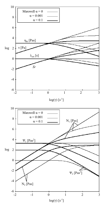
Figure 4.151: Effect of α on the Giesekus Model for an Extensional Flow shows the behavior of the Giesekus fluid in an extensional flow.
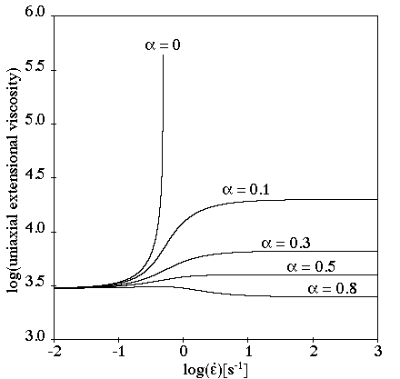
In this case, the steady extensional viscosities are finite. For
small values of  extension thickening occurs, and for large values
extension thinning occurs.
extension thickening occurs, and for large values
extension thinning occurs.
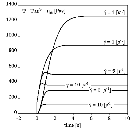
In a transient shear flow (Figure 4.152: Giesekus Model for a Transient Shear Flow), the stress overshoot is less severe than for the PTT model; there are fewer oscillations.
The duration of the transient phase depends on the imposed shear rate (the same behavior as for the PTT model). For a high shear rate, you can observe stress overshoots during the transient phase. With increasing shear rate, the overshoot increases while the final value of the displayed properties decreases. The duration of the transient phases decreases as the shear rate increases.
![]() Rheometry → Fluid
Model → Differential Viscoelastic
Properties → Model →
Fene-P
Rheometry → Fluid
Model → Differential Viscoelastic
Properties → Model →
Fene-P
The FENE-P model is derived from molecular theories and assumes that
the polymer macromolecules are idealized as dumbbells linked with an
elastic connector or spring and suspended in a Newtonian solvent of
viscosity  . Unlike in the Maxwell model, however, the springs are
allowed only a finite extension, so that the energy of deformation of
the dumbbell becomes infinite for a finite value of the spring
elongation. This model predicts a realistic shear thinning of the fluid
and a first normal-stress difference that is quadratic for low shear
rates and has a lower slope for high shear rates.
. Unlike in the Maxwell model, however, the springs are
allowed only a finite extension, so that the energy of deformation of
the dumbbell becomes infinite for a finite value of the spring
elongation. This model predicts a realistic shear thinning of the fluid
and a first normal-stress difference that is quadratic for low shear
rates and has a lower slope for high shear rates.
The FENE-P model computes  from
from
 | (4–56) |
where the configuration tensor  is computed from
 | (4–57) |
and  is the ratio of the maximum length of the spring
to its length at rest:
is the ratio of the maximum length of the spring
to its length at rest:
 | (4–58) |
 is an equilibrium length that corresponds to rigid
motion (in this case,
is an equilibrium length that corresponds to rigid
motion (in this case,  =0 and the tension in the connector equals the
Brownian forces).
=0 and the tension in the connector equals the
Brownian forces).  is the maximum allowable dumbbell length. Figure 4.153: Dumbbell Definitions for the FENE-P Model shows
how the distance between dumbbells is based on the relative position
of both ends.
is the maximum allowable dumbbell length. Figure 4.153: Dumbbell Definitions for the FENE-P Model shows
how the distance between dumbbells is based on the relative position
of both ends.
 is always greater than 1. As
  becomes infinite, the FENE-P model reduces to the
upper-convected Maxwell model.
becomes infinite, the FENE-P model reduces to the
upper-convected Maxwell model.
 is computed (optionally) from Equation 4–47.
 in Equation 4–56 is the partial
viscosity, while
in Equation 4–56 is the partial
viscosity, while  in Equation 4–47 is the additional viscosity.
The motion of the dumbbells is the result of hydrodynamic,
Brownian, and spring forces.  represents the tension in the spring (spring
forces) and the Brownian motion.
represents the tension in the spring (spring
forces) and the Brownian motion.  represents the Newtonian (hydrodynamic) forces.
See 1 for additional information about the FENE-P model.
The units for the parameters and their names in the Fluent Materials Processing interface are as follows:
| Parameter | Name in Fluent Materials Processing | Mass | Length | Time |
|---|---|---|---|---|
 | Partial Viscosity [Pa s] | 1 | –1 | –1 |
 | Relaxation Time [s] | – | – | 1 |
 | Additional Viscosity [Pa s] | 1 | –1 | –1 |
 | L^2 | – | – | – |
By default,  is set to 1 while
  is set to 10-16.
 is set to 1.1 and
  to 0. Additionally, by default, Number
of Relaxation Modes is set to 1. You can select multiple
relaxation modes, in which case multiple sets of parameters will
have to be specified (
to 0. Additionally, by default, Number
of Relaxation Modes is set to 1. You can select multiple
relaxation modes, in which case multiple sets of parameters will
have to be specified ( ,
,  ,
,  ).
).
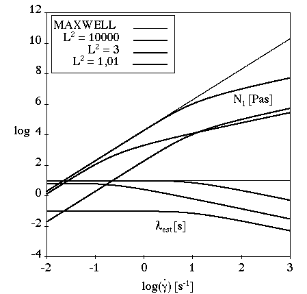
The behavior of the FENE-P model with small values of
 for a simple shear flow is illustrated in Figure 4.154: Effect of Small Values of L^2 on the FENE-P Model for Shear
Flow.
Shear thinning occurs with this model, and for large values of shear
rate, the slope is –2/3. Therefore the addition of a
Newtonian viscosity component is not required for stability. The
first normal-stress difference is non-quadratic, and the second
normal-stress difference is 0. The cut-off appears sooner when
for a simple shear flow is illustrated in Figure 4.154: Effect of Small Values of L^2 on the FENE-P Model for Shear
Flow.
Shear thinning occurs with this model, and for large values of shear
rate, the slope is –2/3. Therefore the addition of a
Newtonian viscosity component is not required for stability. The
first normal-stress difference is non-quadratic, and the second
normal-stress difference is 0. The cut-off appears sooner when
 decreases, down to a value of 3. No asymptotic
behavior is observed. For low values of shear rate,
decreases, down to a value of 3. No asymptotic
behavior is observed. For low values of shear rate,  decreases as
  decreases.
The behavior of the FENE-P model with large values of
 for a simple shear flow is illustrated in Figure 4.155: Effect of Large Values of L^2 on the FENE-P Model for Shear
Flow.
for a simple shear flow is illustrated in Figure 4.155: Effect of Large Values of L^2 on the FENE-P Model for Shear
Flow.
For large values of  , the FENE-P model is observed to exhibit
Maxwellian behavior: quadratic first normal-stress difference and
, the FENE-P model is observed to exhibit
Maxwellian behavior: quadratic first normal-stress difference and
 close to
  . For
. For  close to 1, Newtonian behavior is observed:
quadratic but small first normal-stress difference,
close to 1, Newtonian behavior is observed:
quadratic but small first normal-stress difference,  tends toward 0, cut-off occurs at high shear
rates. For low shear rates,
tends toward 0, cut-off occurs at high shear
rates. For low shear rates,
 | (4–59) |
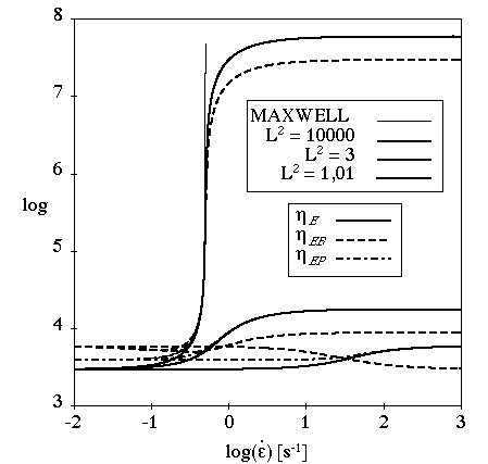
For extensional flows,  controls the extensional viscosity. As shown in
Figure 4.156: Effect of L^2 on the FENE-P Model for Extensional
Flow,
the extensional viscosities are finite. For large values of
controls the extensional viscosity. As shown in
Figure 4.156: Effect of L^2 on the FENE-P Model for Extensional
Flow,
the extensional viscosities are finite. For large values of
 , the FENE-P model is observed to exhibit
Maxwellian behavior: the extensional viscosities are very high for
, the FENE-P model is observed to exhibit
Maxwellian behavior: the extensional viscosities are very high for
 . For
. For  close to 1, Newtonian behavior is observed: the
extensional viscosities are constant.
close to 1, Newtonian behavior is observed: the
extensional viscosities are constant.
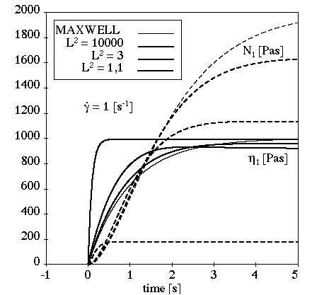
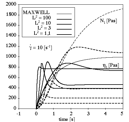
The behavior of the FENE-P model for a transient shear flow is
shown in Figure 4.157: Effect of Large Values of L^2 on the FENE-P Model for
Transient Shear Flow and Figure 4.158: Effect of Mid-Range Values of L^2 on the FENE-P Model for
Transient Shear Flow. For
high shear rates, the stress overshoots in the transient phase. When
the shear rate increases, the final value and the transient phase
decrease while the overshoot increases. For large values of
 , the FENE-P model is observed to exhibit
Maxwellian behavior: no stress overshoots. For mid-range values of
, the FENE-P model is observed to exhibit
Maxwellian behavior: no stress overshoots. For mid-range values of
 , the stress overshoots increase and the transient
phase decreases as
, the stress overshoots increase and the transient
phase decreases as  decreases. For
  close to 1, Newtonian behavior is observed: no
stress overshoots and a short transient phase even for high values
of shear rate.
close to 1, Newtonian behavior is observed: no
stress overshoots and a short transient phase even for high values
of shear rate.
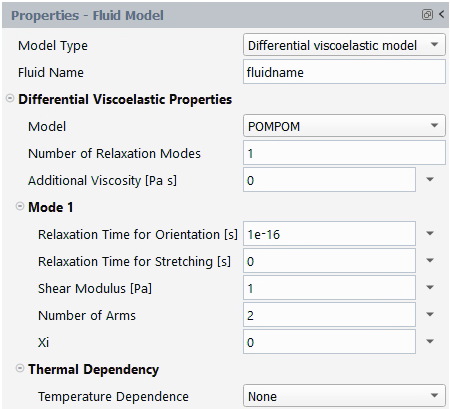
![]() Rheometry → Fluid
Model → Differential Viscoelastic
Properties → Model →
POMPOM
Rheometry → Fluid
Model → Differential Viscoelastic
Properties → Model →
POMPOM
In the POMPOM model, the pom-pom molecule consists of a backbone to
which  arms are connected at both extremities. In a flow, the
backbone may orient in a Doi-Edwards reptation tube consisting of the
neighboring molecules, while the arms may retract into that tube. The
concept of the pom-pom macromolecule makes the model suitable for
describing the behavior of branched polymers. The approximate
differential form of the model is based on equations of macromolecular
orientation, and macromolecular stretching in relation to changes in
orientation.
arms are connected at both extremities. In a flow, the
backbone may orient in a Doi-Edwards reptation tube consisting of the
neighboring molecules, while the arms may retract into that tube. The
concept of the pom-pom macromolecule makes the model suitable for
describing the behavior of branched polymers. The approximate
differential form of the model is based on equations of macromolecular
orientation, and macromolecular stretching in relation to changes in
orientation.
The model, referred to as DCPP (2, 8), allows for a nonzero second normal
stress difference. The DCPP model computes  from an orientation tensor,
  and a stretching scalar
  (states variables), on the basis of the following
algebraic equation:
(states variables), on the basis of the following
algebraic equation:
 | (4–60) |
where  is the shear modulus and
  is a nonlinear material parameter (the nonlinear
material parameter will be introduced later on). The state variables
is a nonlinear material parameter (the nonlinear
material parameter will be introduced later on). The state variables
 and
and  are computed from the following differential
equations:
are computed from the following differential
equations:
 | (4–61) |
 | (4–62) |
In these equations,  and
and  are the relaxation times associated with the
orientation and stretching mechanisms respectively. In the last
equation,
are the relaxation times associated with the
orientation and stretching mechanisms respectively. In the last
equation,  characterizes the number of dangling arms (or
priority) at the extremities of the pom-pom molecule or segment. It is
an indication of the maximum stretching that the molecule can undergo,
and therefore of a possible strain hardening behavior.
characterizes the number of dangling arms (or
priority) at the extremities of the pom-pom molecule or segment. It is
an indication of the maximum stretching that the molecule can undergo,
and therefore of a possible strain hardening behavior.  can be obtained from the elongational behavior.
 is a nonlinear parameter that has enabled the
introduction of a non-vanishing second normal stress difference in the
DCPP model.
is a nonlinear parameter that has enabled the
introduction of a non-vanishing second normal stress difference in the
DCPP model.
A multi-mode DCPP model can also be defined. Each contribution
 will involve an orientation tensor
  and a stretching variable
  . A few guidelines are required for the determination
of the several linear and nonlinear parameters.
. A few guidelines are required for the determination
of the several linear and nonlinear parameters.
Consider a multi-mode DCPP model characterized by  modes sorted with increasing values of relaxation
times
modes sorted with increasing values of relaxation
times  (increasing seniority). The linear parameters
 and
and  characterizing the linear viscoelastic behavior of the
model can be determined with the usual procedure.
characterizing the linear viscoelastic behavior of the
model can be determined with the usual procedure.
Then the relaxation times ( ) for stretching should be determined. Depending on the
average number of entanglements of backbone section, the ratio
) for stretching should be determined. Depending on the
average number of entanglements of backbone section, the ratio
 should be within the range of 2 to 10. For a
completely unentangled polymer segment, you may accept the physical
limit of
should be within the range of 2 to 10. For a
completely unentangled polymer segment, you may accept the physical
limit of  =
= .
.  should also satisfy the constraint
  , since
  sets the fundamental diffusion time for the branch
point controlling the relaxation of polymer segment (
sets the fundamental diffusion time for the branch
point controlling the relaxation of polymer segment ( ).
).
The parameter  indicating the number of dangling arms (or priority)
at the extremities of a pom-pom segment
indicating the number of dangling arms (or priority)
at the extremities of a pom-pom segment  , also indicates the maximum stretching that can be
undergone by that segment, and therefore its possible strain hardening
behavior. For a multi-mode DCPP model, both seniority and priority are
assumed to increase together towards the inner segments; hence
, also indicates the maximum stretching that can be
undergone by that segment, and therefore its possible strain hardening
behavior. For a multi-mode DCPP model, both seniority and priority are
assumed to increase together towards the inner segments; hence
 should also increase with
  . The parameter
  can be obtained from the elongational behavior.
 is a fifth set of nonlinear parameters that control
the ratio of second to first normal stress differences. The value of
parameter
is a fifth set of nonlinear parameters that control
the ratio of second to first normal stress differences. The value of
parameter  should range between 0 and 1. For moderate values,
 corresponds to twice the ratio of the second to the
first normal stress difference, and may decrease with increasing
seniority.
corresponds to twice the ratio of the second to the
first normal stress difference, and may decrease with increasing
seniority.
As for other viscoelastic models, a purely viscous component
 can be added to the viscoelastic component
 , in order to get the total extra-stress tensor:
 | (4–63) |
where
 | (4–64) |
where  is the rate-of-deformation tensor and
  is the additional (Newtonian) viscosity.
The units for the parameters and their names in the Fluent Materials Processing interface are as follows:
| Parameter | Name in Fluent Materials Processing | Mass | Length | Time |
|---|---|---|---|---|
 | Additional Viscosity [Pa s] | 1 | –1 | –1 |
 | Relaxation Time for Orientation [s] | - | - | 1 |
 | Shear Modulus [Pa] | 1 | –1 | –2 |
 | Relaxation Time for Stretching [s] | - | - | 1 |
 | Number of Arms | - | - | - |
 | Xi | - | - | - |
By default, the shear modulus and the relaxation time for
orientation are respectively initialized to 1 and
10-16. The relaxation time for stretching
and xi are initialized to 0 while Number of
Arms is initialized to 2. Additionally, by default,
Number of Relaxation Modes is set to 1. You can
select multiple relaxation modes, in which case multiple sets of
parameters will have to be specified ( ,
,  ,
,  ,
,  ,
,  ).
).
Figure 4.159: Effect of Parameter ξ for Steady Shear Flow
shows the steady viscometric behavior of a single mode DCPP fluid
model for various values of the parameter  . For the present illustration, the shear modulus
equals 1000, while the relaxation times for orientation and
stretching have been assigned the values 1 and 0.5, respectively. As
can be seen, constant viscosity and quadratic first normal stress
difference are obtained at low shear rates. Nonlinear behavior is
found beyond
. For the present illustration, the shear modulus
equals 1000, while the relaxation times for orientation and
stretching have been assigned the values 1 and 0.5, respectively. As
can be seen, constant viscosity and quadratic first normal stress
difference are obtained at low shear rates. Nonlinear behavior is
found beyond  . We also find that an increasing value of
 enforces the nonlinear behavior, while it also
generates a non-vanishing second normal stress difference. The other
nonlinear parameters
enforces the nonlinear behavior, while it also
generates a non-vanishing second normal stress difference. The other
nonlinear parameters  and
and  have actually a negligible influence on the
viscometric properties.
have actually a negligible influence on the
viscometric properties.
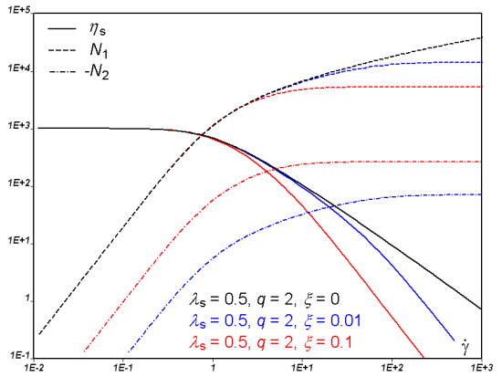
In Figure 4.160: Effect of Parameter q on Steady Elongation Viscosity, the steady elongation viscosity of a single mode DCPP fluid
model for increasing values of  is displayed. For the continuous curves, the shear
modulus equals 1000, while the relaxation times for orientation and
stretching have been assigned the values 1 and 0.5, respectively.
Also, the nonlinear parameter
is displayed. For the continuous curves, the shear
modulus equals 1000, while the relaxation times for orientation and
stretching have been assigned the values 1 and 0.5, respectively.
Also, the nonlinear parameter  is equal to 0.1. As is known for the DCPP model,
and more generally for pom-pom models, the parameter
is equal to 0.1. As is known for the DCPP model,
and more generally for pom-pom models, the parameter  is an indication of branching, and therefore of
strain hardening in elongation. As can be seen from Figure 4.160: Effect of Parameter q on Steady Elongation Viscosity, the
elongation viscosity increases when the strain
is an indication of branching, and therefore of
strain hardening in elongation. As can be seen from Figure 4.160: Effect of Parameter q on Steady Elongation Viscosity, the
elongation viscosity increases when the strain  rate is larger than
  , and the strain hardening is enhanced for
increasing values of
, and the strain hardening is enhanced for
increasing values of  . The figure also shows the steady elongation
viscosity obtained for
. The figure also shows the steady elongation
viscosity obtained for  as well as for
  . As can be seen, the influence of these parameters
on the steady elongation viscosity remains moderate as compared to
that of parameter
. As can be seen, the influence of these parameters
on the steady elongation viscosity remains moderate as compared to
that of parameter  .
.
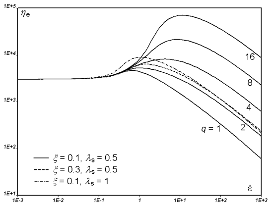
Finally, Figure 4.161: Effect of Parameter q on Transient Elongation Viscosity for
Different Values of the Elongation Rate shows the transient elongation viscosity of
various single-mode DCPP fluid model characterized by different
branching levels ( ), at elongation rates
  successively equal to 0.1, 1 and 10. We find that
all curves collapse at low strain rate (0.1), while they markedly
differ at high strain rate (10).
successively equal to 0.1, 1 and 10. We find that
all curves collapse at low strain rate (0.1), while they markedly
differ at high strain rate (10).
Figure 4.161: Effect of Parameter q on Transient Elongation Viscosity for Different Values of the Elongation Rate
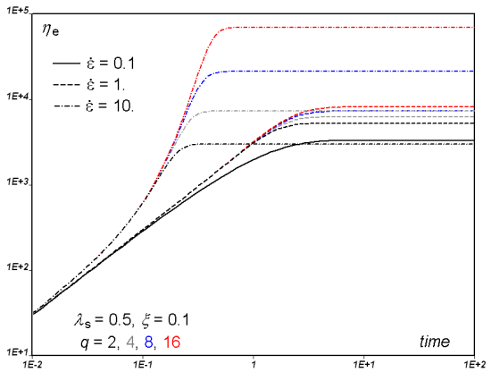
![]() Rheometry → Fluid
Model → Differential Viscoelastic
Properties → Model →
Leonov
Rheometry → Fluid
Model → Differential Viscoelastic
Properties → Model →
Leonov
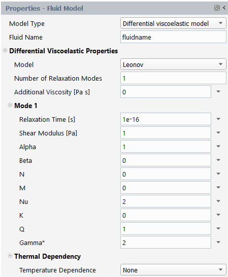
Elastomers are usually filled with carbon black and/or silicate. From the point of view of morphology, macromolecules at rest are trapped by particles of carbon black, via electrostatic van der Waals forces. Under a deformation field, electrostatic bonds can break, and macromolecules become free, while a reverse mechanism may develop when the deformation ceases. You can therefore be facing a macromolecular system consisting of trapped and free macromolecules, with a reversible transition from one state to the other one.
Leonov and Simhambhatla have developed a rheological model (9, 3) for the simultaneous prediction of the behavior for trapped and free macromolecular chains. This model for filled elastomers involves two tensor quantities and a scalar one. These tensor quantities focus respectively on the behavior of the free and trapped macromolecular chains of the elastomer, while the scalar quantity quantifies the degree of structural damage (debonding factor). The model exhibits a yielding behavior. It is intrinsically nonlinear, as the nonlinear response develops and is observable at early deformations.
In a single-mode approach, the total stress tensor  can be decomposed as the sum of free and trapped
contributions as follows:
can be decomposed as the sum of free and trapped
contributions as follows:
 | (4–65) |
As for other viscoelastic models, a purely viscous component
 is added to the viscoelastic components in order to
get the total extra-stress tensor:
is added to the viscoelastic components in order to
get the total extra-stress tensor:
 | (4–66) |
where  is the rate-of-deformation tensor and
  is the viscosity.
In Equation 4–65,
subscripts  and
and  respectively refer to the free and trapped parts. Each
of these contributions obeys its own equation. In particular, they
invoke their own deformation field described by means of Finger tensors.
respectively refer to the free and trapped parts. Each
of these contributions obeys its own equation. In particular, they
invoke their own deformation field described by means of Finger tensors.
An elastic Finger tensor  is defined for the free chains, which obeys the
following equation:
is defined for the free chains, which obeys the
following equation:
 | (4–67) |
where  is the relaxation time,
  is the unit tensor, while
  and
and  are the first invariant of
  and
and  , respectively, defined as
 | (4–68) |
 | (4–69) |
The implemented material function  that appears in Equation 4–67 is
written as follows:
that appears in Equation 4–67 is
written as follows:
 | (4–70) |
The parameter  must be
  and increases slightly the amount of shear
thinning.
and increases slightly the amount of shear
thinning.
Similarly, an elastic Finger tensor  is defined for the trapped chains, which obeys the
following equation:
is defined for the trapped chains, which obeys the
following equation:
 | (4–71) |
where  and
and  are the first invariant of
  and
and  , respectively, defined as
 | (4–72) |
 | (4–73) |
In the equation for the trapped chains, the variable  quantifies the degree of structural damage (debonding
factor), and is the fraction of the initially trapped chains that are
debonded from the filler particles during flow. The function
quantifies the degree of structural damage (debonding
factor), and is the fraction of the initially trapped chains that are
debonded from the filler particles during flow. The function
 is a structural damage dependent scaling factor for
the relaxation time
is a structural damage dependent scaling factor for
the relaxation time  and is referred to as the “mobility function".
A phenomenological kinetic equation is suggested for  :
:
 | (4–74) |
In Equation 4–74,
 is the local shear rate while
  is the yielding strain. Also,
  is a dimensionless time factor, which may delay or
accelerate debonding.
is a dimensionless time factor, which may delay or
accelerate debonding.
For the mobility function  appearing in Equation 4–71, the
following form has been implemented:
appearing in Equation 4–71, the
following form has been implemented:
 | (4–75) |
The above selection for the mobility function endows the rheological
properties with a yielding behavior. When  is large (or unbounded), the algebraic term dominates
the constitutive equation for
is large (or unbounded), the algebraic term dominates
the constitutive equation for  (Equation 4–71), and the solution is expected to be
 . When
  is vanishing,
  becomes governed by a purely transport equation; this
may lead to numerical troubles when solving a complex steady flow with
secondary motions (vortices). This situation can occur if parameter
becomes governed by a purely transport equation; this
may lead to numerical troubles when solving a complex steady flow with
secondary motions (vortices). This situation can occur if parameter
 is set to zero and under no-debonding situation
(
is set to zero and under no-debonding situation
( ). Therefore, you should impose a small (but nonzero)
value for parameter
). Therefore, you should impose a small (but nonzero)
value for parameter  (by default, we suggest the value 0.05, which is a
reasonable compromise between rheological properties and solver
stability). Based on this, parameter
(by default, we suggest the value 0.05, which is a
reasonable compromise between rheological properties and solver
stability). Based on this, parameter  can be understood as the value of the mobility
function under no-debonding.
can be understood as the value of the mobility
function under no-debonding.
Finally, in order to relate the Finger tensors to the corresponding
stress tensor, potential functions are required. For  and
and  , the following expressions are suggested:
 | (4–76) |
 | (4–77) |
with  and
and  . It is interesting to note that
  has no effect on the shear viscosity, while it
contributes to a decrease of the elongational viscosity. On the other
hand, the parameter
has no effect on the shear viscosity, while it
contributes to a decrease of the elongational viscosity. On the other
hand, the parameter  increases both shear and elongational viscosities.
From there, stress contributions from free and trapped chains in Equation 4–65 are respectively
given by:
increases both shear and elongational viscosities.
From there, stress contributions from free and trapped chains in Equation 4–65 are respectively
given by:
 | (4–78) |
 | (4–79) |
where parameter  is the initial ratio of free to trapped chains in the
system. A vanishing value of
is the initial ratio of free to trapped chains in the
system. A vanishing value of  indicates that all chains are trapped at rest, while a
large value of
indicates that all chains are trapped at rest, while a
large value of  indicates a system that essentially consists of free
chains.
indicates a system that essentially consists of free
chains.
The units for the parameters and their names in the Fluent Materials Processing interface are as follows:
| Parameter | Name in Fluent Materials Processing | Mass | Length | Time |
|---|---|---|---|---|
 | Additional Viscosity [Pa s] | 1 | –1 | –1 |
 | Relaxation Time [s] | - | - | 1 |
 | Shear Modulus [Pa] | 1 | –1 | –2 |
 | Alpha | - | - | - |
 | Beta | - | - | - |
 | N | - | - | - |
 | M | - | - | - |
 | Nu | - | - | - |
 | K | - | - | - |
 | Q | - | - | - |
 | Gamma* | - | - | - |
By default,  is set to 0,
  is set to 10-16,
 and
and  are set to 1,
  ,
,  and
and  are set to 0,
  is set to 2,
  is set to 0,
  is set to 1 and
  is set to 2. Additionally, by default,
Number of Relaxation Modes is set to 1. You can
select multiple relaxation modes, in which case multiple sets of
parameters will have to be specified (
is set to 2. Additionally, by default,
Number of Relaxation Modes is set to 1. You can
select multiple relaxation modes, in which case multiple sets of
parameters will have to be specified ( ,
,  ,
,  ,
,  ,
,  ,
,  ,
,  ,
,  ,
,  ,
,  ).
).
From the point of view of rheology and numerical simulation, for single- and multi-mode fluid models, a purely viscous contribution must be added to the total extra-stress tensor. Actually, this is largely motivated by the fact that the matrix of the discretized system can be singular when all fields are initialized to values that correspond to the solution at rest. Hence, the first or only mode will always be accompanied by a Newtonian contribution, whose corresponding viscosity value received a unit default value. This value can be modified you.
Also, as suggested above, a non-vanishing value  should be selected for the mobility function under
no-debonding.
should be selected for the mobility function under
no-debonding.
As can be seen, next to parameters  and
and  controlling the linear properties, the model
involves two functions and several nonlinear parameters. In a single
mode approach, the influence of these parameters on the viscometric
and elongational properties can be easily identified, and
appropriate values can be selected accordingly. By default, the
nonlinear parameters are assigned values that are relevant from the
point of view of rheology. In a multi-mode approach, in order to
facilitate the definition of a flow case, corresponding nonlinear
parameters should preferably be identical for each mode.
controlling the linear properties, the model
involves two functions and several nonlinear parameters. In a single
mode approach, the influence of these parameters on the viscometric
and elongational properties can be easily identified, and
appropriate values can be selected accordingly. By default, the
nonlinear parameters are assigned values that are relevant from the
point of view of rheology. In a multi-mode approach, in order to
facilitate the definition of a flow case, corresponding nonlinear
parameters should preferably be identical for each mode.
In simple shear flow, the Leonov model exhibits shear thinning,
which is slightly affected by some parameters. Figure 4.162: Shear Viscosity of the Leonov Model with Parameters G=1000,
λ=1, q=1, β=0, ν=2, γ*=2, and α=1, k=n=m=0
(continuous lines). shows
that an increase of the parameter  (initial ratio of free to trapped chains) slightly
decreases the shear viscosity at low shear rates. This can be easily
understood if you consider, for example, that when
(initial ratio of free to trapped chains) slightly
decreases the shear viscosity at low shear rates. This can be easily
understood if you consider, for example, that when  =0, the material consists only of trapped chains at
rest. The figure also shows that parameter
=0, the material consists only of trapped chains at
rest. The figure also shows that parameter  increases the shear viscosity at high shear rates,
while parameter
increases the shear viscosity at high shear rates,
while parameter  has a very limited influence. Finally, as can be
seen in Figure 4.162: Shear Viscosity of the Leonov Model with Parameters G=1000,
λ=1, q=1, β=0, ν=2, γ*=2, and α=1, k=n=m=0
(continuous lines)., shear viscosity curves do not show a plateau
at low shear rates. This is the fingerprint of the yielding behavior
of the fluid model, which is controlled by the value of the mobility
function under no-debonding (parameter
has a very limited influence. Finally, as can be
seen in Figure 4.162: Shear Viscosity of the Leonov Model with Parameters G=1000,
λ=1, q=1, β=0, ν=2, γ*=2, and α=1, k=n=m=0
(continuous lines)., shear viscosity curves do not show a plateau
at low shear rates. This is the fingerprint of the yielding behavior
of the fluid model, which is controlled by the value of the mobility
function under no-debonding (parameter  ). If
). If  increases, the viscosity curves exhibit a plateau
at low shear rates. However, as can be seen in the insert, this does
not affect the behavior at high shear rates, while it may improve
the stability of the solver.
increases, the viscosity curves exhibit a plateau
at low shear rates. However, as can be seen in the insert, this does
not affect the behavior at high shear rates, while it may improve
the stability of the solver.
Figure 4.162: Shear Viscosity of the Leonov Model with Parameters G=1000, λ=1, q=1, β=0, ν=2, γ*=2, and α=1, k=n=m=0 (continuous lines).
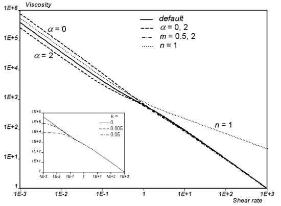
Dashed and dashed-dotted lines show the viscosity for the value of the parameters as indicated. The insert shows the viscosity curves obtained for various values of the mobility function under no-debonding (parameter k).
Figure 4.163: First Normal Stress Difference of the Leonov Model with
Parameters G=1000, λ=1, q=1, β=0, ν=2, γ*=2, and
α=1, k=n=m=0 (continuous lines). shows that similar trends are found for the
first normal stress difference. Figure 4.163: First Normal Stress Difference of the Leonov Model with
Parameters G=1000, λ=1, q=1, β=0, ν=2, γ*=2, and
α=1, k=n=m=0 (continuous lines).
shows that an increase of the parameter  slightly decreases the first normal stress
difference at all shear rates. The figure also shows that parameter
slightly decreases the first normal stress
difference at all shear rates. The figure also shows that parameter
 increases the first normal stress difference at
all shear rates, while parameter
increases the first normal stress difference at
all shear rates, while parameter  decreases it at high shear rates. Finally, as can
be seen, the first normal stress difference shows a plateau at low
shear rates; this is a counterpart of the yielding behavior of the
fluid model, which is also controlled by the value of the mobility
function under no-debonding (parameter
decreases it at high shear rates. Finally, as can
be seen, the first normal stress difference shows a plateau at low
shear rates; this is a counterpart of the yielding behavior of the
fluid model, which is also controlled by the value of the mobility
function under no-debonding (parameter  ). If
). If  increases, the first normal stress difference
exhibit a quadratic behavior at low shear rates; however, as can be
seen in the insert, this does not affect the behavior at high shear
rates, while it may improve the stability of the solver.
increases, the first normal stress difference
exhibit a quadratic behavior at low shear rates; however, as can be
seen in the insert, this does not affect the behavior at high shear
rates, while it may improve the stability of the solver.
Figure 4.163: First Normal Stress Difference of the Leonov Model with Parameters G=1000, λ=1, q=1, β=0, ν=2, γ*=2, and α=1, k=n=m=0 (continuous lines).
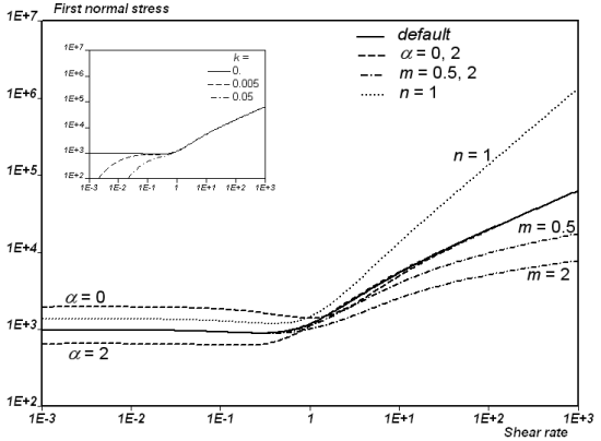
Dashed, dashed-dotted and dotted lines show the first normal
stress difference for the value of the parameters as indicated. The
insert shows the curves of first normal stress difference obtained
for various values of the mobility function under no-debonding
(parameter  ).
).
In simple elongation flow, the Leonov model exhibits marked strain
thinning at low strain rates; it is slightly affected by some
parameters. Figure 4.164: Elongation Viscosity of the Leonov Model with Parameters
G=1000, λ=1, q=1, n=1, ν=2, γ*=2, and α=1,
β=k=m=0 (continuous lines). shows that an increase of the parameter
 (initial ratio of free to trapped chains) slightly
decreases the elongation viscosity at low strain rates. This can be
easily understood if you consider, for example, that when
(initial ratio of free to trapped chains) slightly
decreases the elongation viscosity at low strain rates. This can be
easily understood if you consider, for example, that when
 =0, the material consists only of trapped chains at
rest. The figure also shows that parameter
=0, the material consists only of trapped chains at
rest. The figure also shows that parameter  increases the elongation viscosity at high strain
rates, while parameters
increases the elongation viscosity at high strain
rates, while parameters  and
and  decrease the elongation viscosity. Finally, as can
be seen in Figure 4.164: Elongation Viscosity of the Leonov Model with Parameters
G=1000, λ=1, q=1, n=1, ν=2, γ*=2, and α=1,
β=k=m=0 (continuous lines)., elongation viscosity curves do not show a
plateau. This is the fingerprint of the yielding behavior of the
fluid model, which is controlled by the value of the mobility
function under no-debonding (parameter
decrease the elongation viscosity. Finally, as can
be seen in Figure 4.164: Elongation Viscosity of the Leonov Model with Parameters
G=1000, λ=1, q=1, n=1, ν=2, γ*=2, and α=1,
β=k=m=0 (continuous lines)., elongation viscosity curves do not show a
plateau. This is the fingerprint of the yielding behavior of the
fluid model, which is controlled by the value of the mobility
function under no-debonding (parameter  ). Actually, if
  increases, the elongation viscosity curves exhibit
a plateau at low strain rates. However, as can be seen in the insert
of Figure 4.164: Elongation Viscosity of the Leonov Model with Parameters
G=1000, λ=1, q=1, n=1, ν=2, γ*=2, and α=1,
β=k=m=0 (continuous lines)., this does not really affect the behavior at
high strain rates while it may improve the stability of the solver.
increases, the elongation viscosity curves exhibit
a plateau at low strain rates. However, as can be seen in the insert
of Figure 4.164: Elongation Viscosity of the Leonov Model with Parameters
G=1000, λ=1, q=1, n=1, ν=2, γ*=2, and α=1,
β=k=m=0 (continuous lines)., this does not really affect the behavior at
high strain rates while it may improve the stability of the solver.
Figure 4.164: Elongation Viscosity of the Leonov Model with Parameters G=1000, λ=1, q=1, n=1, ν=2, γ*=2, and α=1, β=k=m=0 (continuous lines).
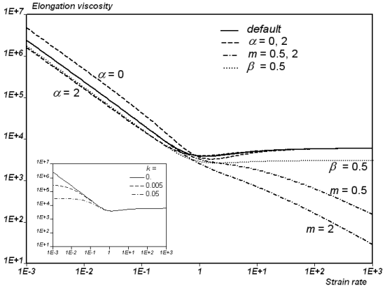
Dashed, dashed-dotted and dotted lines show the elongation
viscosity for the value of the parameters as indicated. The insert
shows the curves of the steady elongation viscosity obtained for
various values of the mobility function under no-debonding
(parameter  ).
).
Note: These curves are not obtained from Fluent Materials Processing Rheometry tool. They result from semi-analytical calculations.
Figure 4.165: Transient Shear Viscosity of the Leonov Model Versus Time, at
Shear Rates Ranging from 10^-2 to 10, With Parameters G=1000,
λ=1, q=1, n=1,, ν=2, γ*=2, and α=1,
β=k=m=n=0, (continuous lines). shows the transient shear viscosity versus time
at shear rates ranging from 10-2 to 10,
for various values of parameters  and
and  . At first, as can be seen, the transient shear
viscosity exhibits an overshoot before reaching the steady value. It
is also interesting to note that the response time decreases when
the shear rate increases. This actually results from the increasing
mobility function under increasing shear rates. Eventually, we find
that parameter
. At first, as can be seen, the transient shear
viscosity exhibits an overshoot before reaching the steady value. It
is also interesting to note that the response time decreases when
the shear rate increases. This actually results from the increasing
mobility function under increasing shear rates. Eventually, we find
that parameter  decreases the elongation viscosity, while the
other parameters have a somewhat less marked influence.
decreases the elongation viscosity, while the
other parameters have a somewhat less marked influence.
Figure 4.165: Transient Shear Viscosity of the Leonov Model Versus Time, at Shear Rates Ranging from 10^-2 to 10, With Parameters G=1000, λ=1, q=1, n=1,, ν=2, γ*=2, and α=1, β=k=m=n=0, (continuous lines).
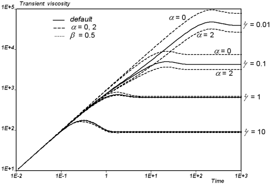
Dashed and dotted lines show the viscosity for the value of the parameters as indicated.
The viscosity in a non-isothermal differential viscoelastic model can be
temperature-dependent. As described in Introduction, the viscosity
will be multiplied by a temperature shift function  . For non-isothermal differential viscoelastic models, the
relaxation time is multiplied by the same temperature shift function.
Temperature-dependent functions available for non-isothermal differential
viscoelastic models are the Arrhenius law, the Arrhenius approximate law,
and the WLF law, all described in Temperature Dependence of Viscosity.
. For non-isothermal differential viscoelastic models, the
relaxation time is multiplied by the same temperature shift function.
Temperature-dependent functions available for non-isothermal differential
viscoelastic models are the Arrhenius law, the Arrhenius approximate law,
and the WLF law, all described in Temperature Dependence of Viscosity.
If you define multiple relaxation modes for your differential viscoelastic fluid, all modes will obey the same constitutive law. Non-linear parameters can be identical or independently specified for each mode, there is no strong argument for one or the other option. For multiple relaxation modes, the viscoelastic stress is written as follows:
 | (4–80) |
A purely viscous component can also be added.
Consider, for example, a fluid being modeled with two relaxation modes as follows:
mode 1: PTT model,
 =0.1 s,
  Pa-s,
Pa-s,  =0.2,
=0.2, 
mode 2: PTT model,
 =1 s,
=1 s,  Pa-s,
Pa-s,  =0.2,
=0.2, 
Figure 4.166: Simple Shear Flow with Multiple Relaxation Times shows
the viscometric behavior for this fluid in a simple shear flow. Here, the
cut-off is controlled by the larger relaxation time, and the slopes of the
curves (for shear rates between 1/ and 1/
 ) are affected.
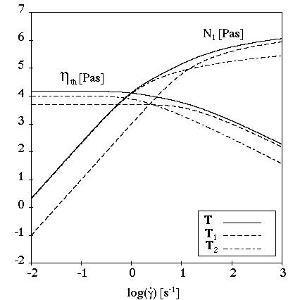
Figure 4.167: Extensional Flow with Multiple Relaxation Times shows
the viscometric behavior for this fluid in an extensional flow. The slopes
of the curves (for extension rates between 1/ and
and  ) are affected.
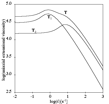
Figure 4.168: Transient Shear Flow with Multiple Relaxation Times shows the viscometric behavior for this fluid in a transient shear flow. The multiple relaxation modes have an effect on the transient phase. In this case, the length of the transient phase depends upon the larger relaxation time. The multiple relaxation modes also affect the overshoot magnitude.
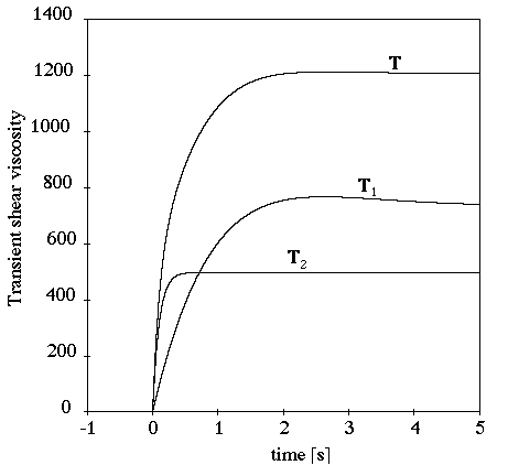
This section describes the following topics:
While the differential models are reasonably suited for 2D and 3D applications, integral constitutive models can be invoked for describing the behavior of melts in applications where the shell model can be used, such as blow molding and thermoforming. These processes are characterized by an elongation kinematics with relatively limited extension deformation.
Note: The integral approach to modeling viscoelastic model is limited to shell models.
For an integral viscoelastic constitutive equation, the extra-stress
tensor  is computed at time
  from the following equation:
 | (4–81) |
where  is the model-specific memory (kernel) function ,
  is the Cauchy-Green strain tensor ,
  is the current time and
  is the metric for time integrals.
For non-isothermal flows,  can be computed from the isothermal constitutive
equation (Equation 4–81), provided that a
modified time scale
can be computed from the isothermal constitutive
equation (Equation 4–81), provided that a
modified time scale  is used for evaluating the strain history:
 | (4–82) |
The modified time scale is related to  through the following equation:
 | (4–83) |
where  is the shift function, which can be obtained from
steady-state shear-viscosity curves at different temperatures. This is
the principle of time-temperature equivalence.
is the shift function, which can be obtained from
steady-state shear-viscosity curves at different temperatures. This is
the principle of time-temperature equivalence.
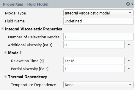
To specify an integral viscoelastic model, select .
![]() Rheometry → Fluid
Model → Model Type
Rheometry → Fluid
Model → Model Type
Specify an appropriate Fluid Name.
Specify Number of Relaxation Modes and Additional Viscosity [Pa s].
Specify Relaxation Time [s] and the Partial Viscosity [Pa s].
Finally, select the law and parameters for the Thermal Dependency.
See Non-Automatic Fitting and Automatic Fitting for information about where and how the material data specification occurs in the non-automatic and automatic fitting procedures, respectively.
See Integral Viscoelastic Models and Temperature Dependence of Viscosity for details about the parameters and characteristics of each fluid model.
The Integral viscoelastic model is primarily dedicated for the simulation of processes like blow molding and thermoforming. These processes involve a kinematics characterized by extension with a bounded deformation amplitude, while shear is absent. Therefore, damping functions are discarded. Linear properties are often sufficient for characterizing the behavior of the melt in such processes. The linear spectrum already allows the prediction of strain hardening and since deformation involved in the shaping processes are often bounded to Hencky strain up to 1 or 2, it is not necessary to mimic the behavior beyond these values.
![]() Rheometry → Fluid
Model → Thermal
Dependency → Temperature
Dependence
Rheometry → Fluid
Model → Thermal
Dependency → Temperature
Dependence
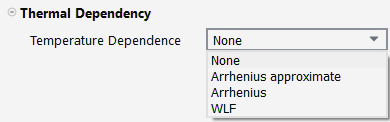
Three models are available for the temperature shift function
 in Equation 4–83: the Arrhenius law, the Arrhenius approximate law,
and the WLF law, all described in Temperature Dependence of Viscosity. It is also
possible to eliminate the temperature dependence using a temperature shift
function equal to 1.
in Equation 4–83: the Arrhenius law, the Arrhenius approximate law,
and the WLF law, all described in Temperature Dependence of Viscosity. It is also
possible to eliminate the temperature dependence using a temperature shift
function equal to 1.
One of the interesting features of viscoelastic model simulations is the prediction of extrudate swelling, which can be larger than their Newtonian counterparts. Running complex 3D flows with a rheologically sophisticated model, however, can be computationally expensive. Therefore, a more simplified approach is needed: one in which you can qualitatively predict the extrudate free surface. This approach is referred to as the “simplified viscoelastic model" or the “light viscoelastic model".
This section describes the following topics:
It is known that the first normal stress difference is mainly responsible
for enhanced extrudate swell in extrusion flow. This is typically a
viscoelastic property. With respect to this, the simplified viscoelastic
model is an extension of existing Newtonian fluid models, where a normal
stress difference has been incorporated into the force balance. That is, in
simple shear flow along the first axis and with a shear rate  , the total extra-stress tensor
  is given by:
 | (4–84) |
In this tensor,  is the shear stress component, which involves the shear
rate dependent viscosity
is the shear stress component, which involves the shear
rate dependent viscosity  . Several laws are available for describing the shear
viscosity (see Generalized Newtonian Model
for more details), for instance, the constant law (Equation 4–30), the Bird-Carreau
law (Equation 4–31),
the Power law (Equation 4–32), the Cross law (Equation 4–37), the modified Cross law (Equation 4–38), and the
Carreau-Yasuda law (Equation 4–39).
. Several laws are available for describing the shear
viscosity (see Generalized Newtonian Model
for more details), for instance, the constant law (Equation 4–30), the Bird-Carreau
law (Equation 4–31),
the Power law (Equation 4–32), the Cross law (Equation 4–37), the modified Cross law (Equation 4–38), and the
Carreau-Yasuda law (Equation 4–39).
The first normal stress is given by  . This quantity involves the viscoelastic variable
 , a quantity
  that can be referred to as the first normal viscosity, and
a weighting coefficient
that can be referred to as the first normal viscosity, and
a weighting coefficient  .
.
The viscoelastic variable  obeys a transport equation that involves a characteristic
or relaxation time
obeys a transport equation that involves a characteristic
or relaxation time  and is given by:
 | (4–85) |
The equation is such that you recover the solution  in simple shear flow. The first normal viscosity
 found in Equation 4–84 is described by means of functions similar to those
available for the shear viscosity
found in Equation 4–84 is described by means of functions similar to those
available for the shear viscosity  , where
  is presently replaced by
  . In order to facilitate the set up of a flow simulation
involving the simplified viscoelastic model, identical dependences for
. In order to facilitate the set up of a flow simulation
involving the simplified viscoelastic model, identical dependences for
 and
and  are considered by default. However, it is important to
note that different functions can be selected for the shear and first normal
viscosities.
are considered by default. However, it is important to
note that different functions can be selected for the shear and first normal
viscosities.
Three algebraic models are available for the relaxation time function:
Constant relaxation
Bird-Carreau law
Power law
Finally, for non-isothermal flows, temperature dependence laws can be selected for the shear and first normal viscosities (see Temperature Dependence of Viscosity for more details). For instance, there is the Arrhenius law Equation 4–42), the approximate Arrhenius law (Equation 4–43), and the WLF law (Equation 4–45).
When defining a non-isothermal case, a single function is used to describe
the temperature dependence of the material functions  ,
,  ,
,  , and optionally of
  .
.
The simplified viscoelastic model is mainly an empirical construction. The key ingredient is the normal stress property that is introduced for the prediction of swelling. Although it is possible to qualitatively relate the swelling and the first normal stress difference, a quantitative relationship is not obvious. Methodologies have to be identified and developed for the determination of material functions and parameters. A stepwise technique is recommended for this purpose.
Note that the simplified viscoelastic model has been developed and implemented mainly for the simulation of 3D extrusion flows, therefore including the prediction of extrudate swelling. Therefore, it is acceptable to use cylindrical extrudate swelling data for the identification of the specific model properties.
As seen above, the simplified viscoelastic model involves three material
functions and a parameter: the shear viscosity  , the first normal viscosity
  , the relaxation time
  , and a weighting coefficient
  . Typically, usual viscosity data should be used for
identifying the shear viscosity function. In most situations, shear thinning
is experimentally observed, and algebraic relationships such as power law,
Bird-Carreau, or Cross laws will be good candidates. However, it is
recommended that you consider a law that exhibits a zero-shear plateau if
regions of no-deformation are expected over the flow domain.
. Typically, usual viscosity data should be used for
identifying the shear viscosity function. In most situations, shear thinning
is experimentally observed, and algebraic relationships such as power law,
Bird-Carreau, or Cross laws will be good candidates. However, it is
recommended that you consider a law that exhibits a zero-shear plateau if
regions of no-deformation are expected over the flow domain.
Important: The parameters of the shear viscosity  can be fitted automatically in Fluent Materials Processing based on
experimental steady shear viscosity curve(s), as for a generalized
Newtonian model. The other parameters of the model cannot be fitted in
Fluent Materials Processing. Note that if rheometric curves are drawn in the chart, only
the Newtonian part of the model is seen.
can be fitted automatically in Fluent Materials Processing based on
experimental steady shear viscosity curve(s), as for a generalized
Newtonian model. The other parameters of the model cannot be fitted in
Fluent Materials Processing. Note that if rheometric curves are drawn in the chart, only
the Newtonian part of the model is seen.
Next, a function and material parameters should be selected for the first
normal viscosity  . By default, a relationship identical to the selected
shear viscosity
. By default, a relationship identical to the selected
shear viscosity  is considered, as this appears to be a reasonable choice,
at least at first. Of course, this default selection can be revised
subsequently. The power law, which exhibits unbounded values under zero
deformation, should be avoided if large regions of no deformation are
expected. Instead, functions that exhibit a plateau, such as the
Bird-Carreau laws, should be preferred.
is considered, as this appears to be a reasonable choice,
at least at first. Of course, this default selection can be revised
subsequently. The power law, which exhibits unbounded values under zero
deformation, should be avoided if large regions of no deformation are
expected. Instead, functions that exhibit a plateau, such as the
Bird-Carreau laws, should be preferred.
Eventually, for the relaxation time  and the weighting coefficient
  , it is suggested to perform a fast 2D simulation of
axisymmetric extrudate swelling, where the effects of the remaining degrees
of freedom are examined. Typically, the weighting coefficient
, it is suggested to perform a fast 2D simulation of
axisymmetric extrudate swelling, where the effects of the remaining degrees
of freedom are examined. Typically, the weighting coefficient
 will control the swelling intensity versus the flow rate,
while the relaxation time function
will control the swelling intensity versus the flow rate,
while the relaxation time function  will control the development of the extrudate diameter
along the jet, and may have a possible influence also on the developed
extrudate geometric attributes. Usually, a constant value or a Bird-Carreau
law can be selected for the relaxation time; the value or zero-shear value
should preferably be in agreement with the typical times involved in the
flow. On the other hand, a series of calculations should be performed with
various values of the weighting coefficient
will control the development of the extrudate diameter
along the jet, and may have a possible influence also on the developed
extrudate geometric attributes. Usually, a constant value or a Bird-Carreau
law can be selected for the relaxation time; the value or zero-shear value
should preferably be in agreement with the typical times involved in the
flow. On the other hand, a series of calculations should be performed with
various values of the weighting coefficient  , where the development of extrudate versus the flow rate
is examined, via an evolution scheme. A comparison with experimental data on
swelling should enable the selection of an appropriate numerical value for
the weighting coefficient
, where the development of extrudate versus the flow rate
is examined, via an evolution scheme. A comparison with experimental data on
swelling should enable the selection of an appropriate numerical value for
the weighting coefficient  .
.
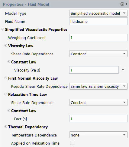
To specify an simplified viscoelastic model, select .
![]() Rheometry → Fluid
Model → Model Type
Rheometry → Fluid
Model → Model Type
The units for the parameters and their names in the Fluent Materials Processing interface are as follows:
| Parameter | Name in Fluent Materials Processing | Mass | Length | Time |
|---|---|---|---|---|
 | Viscosity Law [Pa s] | 1 | –1 | –1 |
 | First Normal Viscosity Law [Pa s] | 1 | –1 | –1 |
 | Relaxation Time Law [s] | - | - | 1 |
 | Weighting Coefficient | - | - | - |
By default, the viscosity, the first normal viscosity, and the relaxation time functions are constant and set to 1. The weighting coefficient is also set to 1.
The simplified viscoelastic model involves three material functions and a
parameter: the shear viscosity  , the normal viscosity
  , the relaxation time
  , and a weighting coefficient
  . Considering the empirical construction of the simplified
viscoelastic model, it is probably more relevant to inspect the behavior
from the point of view of extrusion flow, in particular from the point of
extrudate swelling. As will be seen, the various ingredients may have
opposite effects, and enter in competition with each other.
. Considering the empirical construction of the simplified
viscoelastic model, it is probably more relevant to inspect the behavior
from the point of view of extrusion flow, in particular from the point of
extrudate swelling. As will be seen, the various ingredients may have
opposite effects, and enter in competition with each other.
As is known, shear thinning decreases the extrudate swelling. However, the
other ingredients will usually enhance the swelling. Consider that the
normal and shear viscosities are the same function of their respective
dependence variable; the weighting coefficient and the relaxation time are
to be considered. Actually, selecting a normal viscosity independently with
respect to the shear viscosity will mainly make the analysis more complex
without significantly affecting the general conclusions. The weighting
coefficient  adjusts the intensity of the first normal stress
difference, and will essentially enhance the extrudate swelling. This is
shown in Figure 4.169: Example of axisymmetric extrusion simulation for the simplified
viscoelastic fluid model through a cylindrical tube with a unit
radius., which plots the curve of swelling versus the flow rate
for various simplified viscoelastic fluid models. The continuous lines show
the swelling for various values of the weighting coefficient. Note that the
amount of swelling can significantly be affected. In Figure 4.170: Example of axisymmetric extrusion simulation for the simplified
viscoelastic fluid model through a cylindrical tube with a unit
radius.,
note the development of the free surface versus the axial distance, for
various values of
adjusts the intensity of the first normal stress
difference, and will essentially enhance the extrudate swelling. This is
shown in Figure 4.169: Example of axisymmetric extrusion simulation for the simplified
viscoelastic fluid model through a cylindrical tube with a unit
radius., which plots the curve of swelling versus the flow rate
for various simplified viscoelastic fluid models. The continuous lines show
the swelling for various values of the weighting coefficient. Note that the
amount of swelling can significantly be affected. In Figure 4.170: Example of axisymmetric extrusion simulation for the simplified
viscoelastic fluid model through a cylindrical tube with a unit
radius.,
note the development of the free surface versus the axial distance, for
various values of  . Note that the development versus the position is not
significantly affected be a specific choice of
. Note that the development versus the position is not
significantly affected be a specific choice of  . The relaxation time
  appears in the transport equation for the viscoelastic
variable; consequently it will at first affect the development of the
swelling along the flow direction. This is visible in Figure 4.170: Example of axisymmetric extrusion simulation for the simplified
viscoelastic fluid model through a cylindrical tube with a unit
radius.,
where the dashed lines indicate the development of swelling versus the axial
distance: the development distance increases with the relaxation time, while
actually the amount of swelling is less affected by the relaxation time. As
can be seen in Figure 4.169: Example of axisymmetric extrusion simulation for the simplified
viscoelastic fluid model through a cylindrical tube with a unit
radius., the overall swelling is less affected by the value of
the relaxation time.
appears in the transport equation for the viscoelastic
variable; consequently it will at first affect the development of the
swelling along the flow direction. This is visible in Figure 4.170: Example of axisymmetric extrusion simulation for the simplified
viscoelastic fluid model through a cylindrical tube with a unit
radius.,
where the dashed lines indicate the development of swelling versus the axial
distance: the development distance increases with the relaxation time, while
actually the amount of swelling is less affected by the relaxation time. As
can be seen in Figure 4.169: Example of axisymmetric extrusion simulation for the simplified
viscoelastic fluid model through a cylindrical tube with a unit
radius., the overall swelling is less affected by the value of
the relaxation time.
Figure 4.169: Example of axisymmetric extrusion simulation for the simplified viscoelastic fluid model through a cylindrical tube with a unit radius.
Swelling of an extrudate versus the flow rate, for various values of
 (continuous lines) at
  =0.5 and for various values of
  (dashed lines) at
  . Note that these curves are not obtained from Fluent Materials Processing's
Rheometry tool but rather from
Fluent Materials Processing calculations.
. Note that these curves are not obtained from Fluent Materials Processing's
Rheometry tool but rather from
Fluent Materials Processing calculations.
Figure 4.170: Example of axisymmetric extrusion simulation for the simplified viscoelastic fluid model through a cylindrical tube with a unit radius.
Development of an axisymmetric extrudate versus the axial distance at a
flow rate of 10 (see also Figure 4.169: Example of axisymmetric extrusion simulation for the simplified
viscoelastic fluid model through a cylindrical tube with a unit
radius.), for
various values of  (continuous lines) at
  =0.5 and for various values of
  (dashed lines) at
  =1.2. Note that these curves are not obtained from
Fluent Materials Processing's Rheometry tool but rather from
Fluent Materials Processing calculations.
=1.2. Note that these curves are not obtained from
Fluent Materials Processing's Rheometry tool but rather from
Fluent Materials Processing calculations.
This section describes the following topics:
Depending on the kinematics of the system you are modeling (steady shear flow, steady extensional flow, oscillatory shear flow, and so on), it is possible to compute and plot several viscometric properties in Fluent Materials Processing as they appear under:
![]() Rheometry → Rheometric
Curves → Steady and Oscillatory Curves
Rheometry → Rheometric
Curves → Steady and Oscillatory Curves
and
![]() Rheometry → Rheometric
Curves → Transient Curves
Rheometry → Rheometric
Curves → Transient Curves
which enables you to mimic several rheometry experiments:
The following sections describe various kinematics properties, along with the name of each property as it appears in Fluent Materials Processing.
Steady simple shear flow is characterized by a horizontal velocity field, illustrated in Figure 4.171: Steady Simple Shear Flow and defined as follows:
 | (4–86) |
where  ,
,  , and
, and  are the velocity components in the
  ,
,  , and
, and  directions, respectively, and
  is the constant shear rate, which is equal to
  .
.
On the basis of this flow field, the following properties can be computed:
steady shear stress:

(4–87)
 Rheometry →
Rheometric Curves → Steady and
Oscillatory Curves
Rheometry →
Rheometric Curves → Steady and
Oscillatory Curves Click Shear Stress.
steady shear viscosity:

(4–88)
Rheometry →
Rheometric Curves → Steady and
Oscillatory Curves Click Shear Viscosity.
first normal-stress difference:

(4–89)
Rheometry →
Rheometric Curves → Steady and
Oscillatory Curves Click First Normal Stress Difference.
second normal-stress difference:

(4–90)
Rheometry →
Rheometric Curves → Steady and
Oscillatory Curves Click Second Normal Stress Difference.
first normal-stress coefficient:

(4–91)
Rheometry →
Rheometric Curves → Steady and
Oscillatory Curves Click First Normal Stress Coefficient.
second normal-stress coefficient:

(4–92)
Rheometry →
Rheometric Curves → Steady and
Oscillatory Curves Click Second Normal Stress Coefficient.
recoverable stress:

(4–93)
Rheometry →
Rheometric Curves → Steady and
Oscillatory Curves Click Stress Ratio Sr.
estimated relaxation time:

(4–94)
Rheometry →
Rheometric Curves → Steady and
Oscillatory Curves Click Lambda = Sr / Shear-rate.
Note: Properties given by Equation 4–87 to Equation 4–94 have nonzero values only for viscoelastic fluids. For this reason, these properties are not available in Fluent Materials Processing for generalized Newtonian fluids.
To compute each of these curves, you will need to specify a minimum and
maximum shear rate ( and
and  ), and the number and distribution of sampling points. By
default, 100 points are selected between shear rates of 0.001 and 1000, with a
logarithmic distribution. When thermal dependence is considered, you need to
select the temperature. Note that several temperatures can be selected. These
curves parameters can be specified under:
), and the number and distribution of sampling points. By
default, 100 points are selected between shear rates of 0.001 and 1000, with a
logarithmic distribution. When thermal dependence is considered, you need to
select the temperature. Note that several temperatures can be selected. These
curves parameters can be specified under:
![]() Rheometry → Rheometric
Curves → Curves parameters
Rheometry → Rheometric
Curves → Curves parameters
See Defining Numerical Parameters for information about specifying numerical parameters for viscometric property curves. See Specifying the Curves to be Calculated for information about specifying which curves you want to compute and plot. (Note that, if you use the automatic fitting method, Fluent Materials Processing will automatically compute and plot the curves for all properties for which experimental data curves have been defined.)
Steady extensional flow can be uniaxial, biaxial, or planar. Uniaxial extensional flow is illustrated in Figure 4.172: Uniaxial Extensional Flow and defined as follows:
 | (4–95) |
where  is a constant elongational strain rate.
The corresponding stress distribution can be written as
 | (4–96) |
 | (4–97) |
where  is the uniaxial extensional viscosity.

Biaxial extensional flow is illustrated in Figure 4.173: Biaxial Extensional Flow and defined as follows:
 | (4–98) |
where  is a constant elongational strain rate.
The corresponding stress distribution can be written as
 | (4–99) |
 | (4–100) |
where  is the biaxial extensional viscosity.
Planar extensional flow is illustrated in Figure 4.174: Planar Extensional Flow and defined as follows:
 | (4–101) |
where  is a constant elongational strain rate.

The corresponding stress distribution can be written as
 | (4–102) |
where  is the planar extensional viscosity.
For extensional flow fields, the uniaxial, biaxial, and planar extensional
viscosity curves ( ,
,  , and
, and  ) can be computed. Select ,
and/or , if you want one or
more of these curves to be calculated. These options can be found under:
) can be computed. Select ,
and/or , if you want one or
more of these curves to be calculated. These options can be found under:
![]() Rheometry → Rheometric
Curves → Steady and Oscillatory
Curves
Rheometry → Rheometric
Curves → Steady and Oscillatory
Curves
To compute each of these curves, you will need to specify a minimum and
maximum extensional strain rate ( and
and  ), and the number and distribution of sampling points.
By default, 100 points are selected between strain rates of 0.001 and 1000, with a logarithmic distribution. When thermal dependence is considered, you need to select the temperature. Note that several temperatures can be selected. These curves parameters can be specified under:
![]() Rheometry → Rheometric
Curves → Curves parameters
Rheometry → Rheometric
Curves → Curves parameters
See Defining and Plotting Curves for information about specifying numerical parameters for viscometric property curves. See Specifying the Curves to be Calculated for information about specifying which curves you want to compute and plot. (Note that, if you use the automatic fitting method, Fluent Materials Processing will automatically compute and plot the curves for all properties for which experimental data curves have been defined.)
It is often interesting to examine the response of a viscoelastic material to
a small-amplitude oscillatory shear rate. This flow allows you to investigate
the linear viscoelastic behavior of the material, and yields the storage and
loss moduli,  and
and  . Since small amplitude deformations are considered, storage
and loss moduli for differential and integral models are evaluated as:
. Since small amplitude deformations are considered, storage
and loss moduli for differential and integral models are evaluated as:
 | (4–103) |
For oscillatory shear flow fields, the property curves for the storage and
loss moduli ( and
and  ) can be computed. Select Storage Modulus
G1 and Loss Modulus G2 if you want
Fluent Materials Processing to compute these curves. These options can be found under:
) can be computed. Select Storage Modulus
G1 and Loss Modulus G2 if you want
Fluent Materials Processing to compute these curves. These options can be found under:
![]() Rheometry → Rheometric
Curves → Steady and Oscillatory
Curves
Rheometry → Rheometric
Curves → Steady and Oscillatory
Curves
To compute each of these curves, you will need to specify a
minimum and maximum angular frequency ( and
and  ), and the number and distribution of sampling points.
By default, 100 points are selected between angular frequencies of 0.001 and 1000, with a logarithmic distribution. When thermal dependence is considered, you need to select the temperature. Note that several temperatures can be selected. These curves parameters can be specified under:
![]() Rheometry → Rheometric
Curves → Curves parameters
Rheometry → Rheometric
Curves → Curves parameters
See Defining and Plotting Curves for information about specifying numerical parameters for viscometric property curves. See Specifying the Curves to be Calculated for information about specifying which curves you want to compute and plot. (Note that, if you use the automatic fitting method, Fluent Materials Processing will automatically compute and plot the curves for all properties for which experimental data curves have been defined.)
You can calculate the response of a viscoelastic material to one or more instantaneous variations of shear rate. Two types of transient shear flows can be considered: one can perform an experiment with multiple constant shear rate per interval, or one can simultaneously perform multiple experiments at constant shear rate. The first type allows you to define several types of transient shear flows:


The second type of transient shear flow allows you to define one or multiple transient shear experiments, each being performed with constant shear rate.
For transient shear flow fields, the transient property curves for the properties defined by Equation 4–87 – Equation 4–94 can be computed.
Select Transient Shear Rate, Transient Shear Stress, Transient Shear Viscosity, Transient 1st Normal Stress Difference, Transient 2nd Normal Stress Difference, Transient 1st Normal Stress Coefficient, and/or Transient 2nd Normal Stress Coefficient if you want Fluent Materials Processing to compute one (or more) of these curves.
![]() Rheometry → Rheometric
Curves → Transient Curves
Rheometry → Rheometric
Curves → Transient Curves
To compute each of these curves for experiments with multiple constant shear
rate per interval, you will need to define the desired number of time intervals
during which a constant shear rate is applied. The time interval  is bounded by the time values
  and
and  . All times must be included between the specified minimum and maximum
times, (
. All times must be included between the specified minimum and maximum
times, ( and
and  ). To compute these curves for multiple simultaneous transient
shear experiments with constant shear rate, you only need to specify the number
of experiments and their corresponding shear rate. The number of sampling points
per time interval must also be specified.
). To compute these curves for multiple simultaneous transient
shear experiments with constant shear rate, you only need to specify the number
of experiments and their corresponding shear rate. The number of sampling points
per time interval must also be specified.
![]() Rheometry → Rheometric
Curves → Curves parameters
Rheometry → Rheometric
Curves → Curves parameters
See Defining and Plotting Curves for information about specifying numerical parameters for viscometric property curves. See Specifying the Curves to be Calculated for information about specifying which curves you want to compute and plot. (Note that, if you use the automatic fitting method, Fluent Materials Processing will automatically compute and plot the curves for all properties for which experimental data curves have been defined.)
You may also want to calculate the response of a viscoelastic material to one or more instantaneous variations of strain rate. Three types of transient extensional flows can be considered: one can perform an extensional experiment with a constant stretch velocity, one can perform an extensional experiment with multiple constant strain rate per time interval, or one can simultaneously perform multiple experiments at constant strain rate.
The first type corresponds to a startup elongation experiment where a sample
of initial length L0 is stretched at a constant velocity  . The only required input is the ratio
  /
/ .
.
The second and third types of transient extensional flows correspond to the
types of transient shear flows described in Transient Shear Flow and illustrated by
Figure 4.175: Transient Shear Flows (with the
extensional strain rate  substituted for the shear rate
  ). The velocity field for a transient extensional flow obeys
the same definition as for the corresponding steady extensional flow given in
Steady Extensional Flow.
). The velocity field for a transient extensional flow obeys
the same definition as for the corresponding steady extensional flow given in
Steady Extensional Flow.
In a transient uniaxial extensional flow, the stress difference is
 | (4–108) |
In a biaxial or planar extensional flow, the stress difference is
 | (4–109) |
For transient extensional flow fields, the transient property curves for the properties defined in Steady Extensional Flow can be computed. Select Transient Extensional Rate, Uniaxial Extensional Stress vs. Strain, Uniaxial Extensional Stress vs. Time, Uniaxial Extensional Viscosity vs. Time, Biaxial Extensional Stress vs. Strain, Biaxial Extensional Stress vs. Time, Biaxial Extensional Viscosity vs. Time, and/or Planar Extensional Stress vs. Strain , Planar Extensional Stress vs. Time, Planar Extensional Viscosity vs. Time if you want Fluent Materials Processing to compute these curves.
![]() Rheometry → Rheometric
Curves → Transient Curves
Rheometry → Rheometric
Curves → Transient Curves
To compute each of these curves, you will need to define the desired number of
time intervals during which a constant extensional strain rate is applied. The
time interval  is bounded by the time values
  and
and  . All times must be included between the specified minimum and maximum
times, (
. All times must be included between the specified minimum and maximum
times, ( and
and  ). The number of sampling points per time interval must also be
specified. See Defining Numerical Parameters for information
about specifying numerical parameters for viscometric property curves. See Specifying the Curves to be Calculated for information about specifying
which curves you want to compute and plot. (Note that, if you use the automatic
fitting method, Fluent Materials Processing will automatically compute and plot the curves for
all properties for which experimental data curves have been defined.)
). The number of sampling points per time interval must also be
specified. See Defining Numerical Parameters for information
about specifying numerical parameters for viscometric property curves. See Specifying the Curves to be Calculated for information about specifying
which curves you want to compute and plot. (Note that, if you use the automatic
fitting method, Fluent Materials Processing will automatically compute and plot the curves for
all properties for which experimental data curves have been defined.)
This section explains how to use the automatic and non-automatic fitting methods available in Fluent Materials Processing.
Fluent Materials Processing offers two types of fitting for material data: an automatic method and a non-automatic method. The automatic method is useful for cases where you are primarily interested in directly obtaining the material parameters for a given fluid model. The non-automatic method allows you to perform an in-depth analysis of the properties of a fluid model. If you use the non-automatic method, you can evaluate the sensitivity of the basic viscometric and elongational properties with respect to model parameters. It can also be used when experimental data are obtained on the basis of measurements which are not necessarily accessible via the automatic method (such as transient shear or elongation involving multiple interval with constant shear or strain, respectively). On occasion, the non-automatic method is invoked for fine tuning of automatically fitted parameters. Fluent Materials Processing will try to best fit the parameters of a model without taking solver issues into account. Therefore, it is sometimes necessary to adjust some parameters and fine-tune the fitting to obtain a model which simultaneously mimics the experimental data while being suitable for a complex flow simulation.
Both methods are available for almost all types of models: generalized Newtonian, differential viscoelastic, integral viscoelastic, and simplified viscoelastic. However, for the simplified viscoelastic model, only the viscous part can be fitted. The rheometric curves evaluated by Fluent Materials Processing do not take the additional viscoelastic term of the model into account.
The procedures you need to follow to use the non-automatic and automatic methods are presented in Non-Automatic Fitting and Automatic Fitting, respectively. Details about the inputs for individual fluid models (for example, Bird-Carreau law) are provided in Material Data Parameters, descriptions of the rheological properties for which you can perform fitting are provided in Rheological Properties, and information about controlling the graphical display of the data curves is provided in Defining and Plotting Curves.
This section describes the different types of files that are used during an Fluent Materials Processing session.
During an Fluent Materials Processing session, you will generally need to read and write several kinds of files. Table 4.11: Files Written and Read by Fluent Materials Processing lists the files that Fluent Materials Processing can read and/or write. You can use this table to get an overview of the files you may be using, to find out which codes write a particular file, and to see where to look for more information on each file.
Table 4.11: Files Written and Read by Fluent Materials Processing
| File Type | Created By | Used By | Default Name or Suffix | References |
|---|---|---|---|---|
|
Experimental data curve | External source | Fluent Materials Processing (Rheometry) |
.csv (.crv) | Reading Experimental Data |
|
Calculated property curve | Fluent Materials Processing (Rheometry) | Fluent Materials Processing (Rheometry) | .csv | Saving Calculated Rheometric Curves |
| Material data | Fluent Materials Processing (Setup – possibly with export from Rheometry) | Fluent Materials Processing (Setup – Rheometry via import from Setup) | .mprmat | Reading and Writing Material Data |
This section describes the following topics:
If you use the non-automatic fitting approach in Fluent Materials Processing, you can still read files containing experimental or other data. With the non-automatic fitting approach, you may want to manually and visually search for the optimal parameters to match one or more experimental curves that cannot be fitted automatically. Such experimental data can include transient shear viscosity or transient first normal stress difference vs. time, as well as more complex studies such as stress relaxation, reverse shear flow, and so on.
In this case, the number of accessible experimental curves is greater than for the automatic fitting approach. The approach is identical to that of the automatic fitting method.
![]() Rheometry →
Fitting → Experimental
Curves
Rheometry →
Fitting → Experimental
Curves ![]()
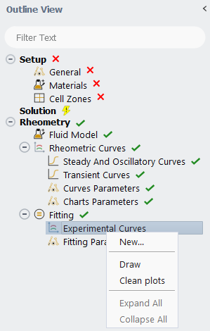
In the Properties - Experimental Curves panel, specify a Name, Filename, Curve Type which corresponds to the experiment and Temperature [K].
The experimental curve types are divided into two categories, those that can be used for both non-automatic and automatic fitting methods, and those that can only be utilized in non-automatic fitting methods. They are separated by an explanatory sentence that explains the specific usage. When a curve can be used for non-automatic fitting method only, a warning is written in the property panel for that curve. However, all of the curves listed above can be employed with the non-automatic fitting method.
Eventually, a title is also generated in the Properties panel, on the basis of the data entered (curve type, temperature, etc.) and which is used for easily identifying the curves in the plots window.
Refer to Files Written or Read by Fluent Materials Processing for more details.
You will need to read your experimental curve data directly into Fluent Materials Processing when using the automatic fitting procedure. The format of the curve file is provided in Reading Experimental Data Curves for the Non-Automatic Fitting Method.
![]() Rheometry →
Fitting → Experimental
Curves
Rheometry →
Fitting → Experimental
Curves ![]()
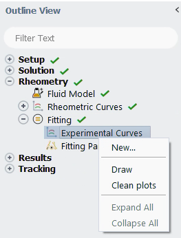
In the Properties - Experimental Curves panel, specify a Name, Filename, Curve Type and the Temperature [K].
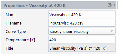
Note: You will need to define at least three types of curves for a viscoelastic model.
You can also define an optional transient uniaxial extensional viscosity curve as well as steady first normal stress difference. You can specify the curves in any order and the type of the curve you import is defined in the Properties panel.
If the file imported contains the viscosity vs. shear-rate curve, click . If it contains the storage modulus vs. angular frequency curve, click . If it contains the loss modulus vs. angular frequency, click . If it contains the transient extensional viscosity curve, click . Lastly, if it contains the first normal stress difference vs. shear rate curve, click .
A title is then generated in the Properties panel, on the basis of the data entered (curve type, temperature, etc.) and which is used for easily identifying the curves in the plots window.
For a , you must specify some flow characteristics:
The Mode (, , ).
The Type, for example, whether the curve is extensional viscosity vs. time or stress vs. strain (
 ), where
  is the initial length of the sample and
 is its current length.
The Regime, for example, whether the sample is stretched at a or .
The Constant Strain Rate or the Initial Strain Rate is required when the sample is stretched at a or at . The initial strain rate
 is defined as the ratio of the constant
extensional velocity
is defined as the ratio of the constant
extensional velocity  to the initial sample length
  .
.
Here too a title is then generated in the Properties panel, on the basis of the data entered (curve type, temperature, etc.) and which is used for easily identifying the curves in the plots window.
Calculated rheometric curves are saved in a Rheometry subfolder located in the Fluent Materials Processing project folder. The filename explicitly refers to the type of property as well as the evaluation ID when Charts Display is set to .
The Rheometry tool primarily communicates outside of
Fluent Materials Processing via ![]() Setup →
Materials.
Setup →
Materials.
In input mode, it can import a rheological model from a material data file
read or created via ![]() Setup →
Materials. It can also directly use data entered via
Setup →
Materials. It can also directly use data entered via
![]() Rheometry → Fluid
Model. In output mode, it can export the created, fitted or
modified rheological model into
Rheometry → Fluid
Model. In output mode, it can export the created, fitted or
modified rheological model into ![]() Setup
→ Materials. To accomplish this,
select:
Setup
→ Materials. To accomplish this,
select:
![]() Rheometry
Rheometry
![]()
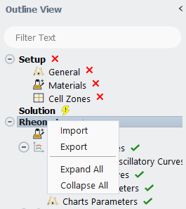
When importing, you can specify the Source Material and Fluid Model to Import.
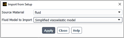
When exporting, you can specify the Target Material and Exported Fluid Model.
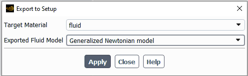
Once the rheological model is configured, you can save the corresponding material data file on disk. For this, right-click the material source in:
![]() Setup →
Materials
Setup →
Materials
![]()
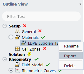
A Select File dialog will open allowing you to specify the Material File name and location where it will be written.
This section explains how to use the non-automatic fitting method in Fluent Materials Processing.
- 4.11.3.3.1. Steps for Non-Automatic Fitting
- 4.11.3.3.2. Specifying the Curves to be Calculated
- 4.11.3.3.3. Defining Curves Parameters
- 4.11.3.3.4. Selecting the Type of Fluid Model
- 4.11.3.3.5. Specifying the Chart Parameters
- 4.11.3.3.6. Performing the Fitting Analysis
- 4.11.3.3.7. Exporting the Results of the Fitting
The steps for non-automatic fitting are as follows:
Fluent Materials Processing allows you to read or define experimental data curves. See Working with Curves. See Reading Experimental Data Curves for the Non-Automatic Fitting Method for a list of available experimental curve types when using the non-automatic fitting method.
Specify which curves you want to calculate (shear viscosity, shear stress, and so on). See Specifying the Curves to be Calculated for details. As mentioned, the non-automatic fitting allows considering experimental data obtained on the basis of measurements which are not necessarily accessible via the automatic method (such as transient shear or elongation involving multiple interval with constant shear or strain, respectively).
Define the numerical parameters for the curve calculation. See Defining Numerical Parameters for details.
Select the fluid model that matches your experimental data best, and define initial values for the associated material parameters. See Selecting the Type of Fluid Model for details.
Modify the value of one material parameter at a time and draw the resulting data curve, until you find the combination that results in a curve most similar to your experimental curve. See Performing the Fitting Analysis for details.
When you are satisfied with the curve fitting, export the result of the fitting to the setup. From there, it can be used for the definition of the simulation and exported into a material data file as well. See Exporting the Results of the Fitting for details.
After you have read or defined your experimental data curve(s), you will need to specify which curves you want Fluent Materials Processing to calculate during the fitting. See Rheological Properties for details about the types of curves that are available. To select the required properties to be calculated and select each of the curves you want:
![]() Rheometry → Rheometric
Curves → Steady And Oscillatory
Curves
Rheometry → Rheometric
Curves → Steady And Oscillatory
Curves
or
![]() Rheometry → Rheometric
Curves → Transient Curves
Rheometry → Rheometric
Curves → Transient Curves
Next, you will need to set some parameters that will be used by Fluent Materials Processing when it calculates the specified curves during the fitting process. For this, select:
![]() Rheometry → Rheometric
Curves → Curve Parameters
Rheometry → Rheometric
Curves → Curve Parameters
In the Properties - Curves Parameters panel, you can specify the number of points used to represent a curve, whether or not to use a linear or logarithmic distribution of points, the range of shear rates for steady properties, the range of angular frequency for the oscillatory properties, the temperature(s), as well as the type of transient shear and elongational flows and the corresponding parameters, as described below.
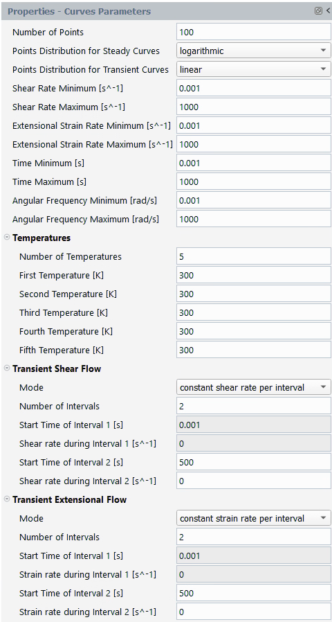
Number of Points
The rheometric curves are discretized into a set of points. Using more points results in a better representation of the curves. The default number of points is 100, which is acceptable for most cases.
Point Distribution For Steady Curves (this also applies to oscillatory curves) - or
These parameters indicate how the calculated points are distributed along the X axis in the equidistant way between successive x values in linear mode, or equidistant between successive log x values in the logarithmic mode.
Point Distribution For Transient Curves - or scale
These parameters indicate how the calculated points are distributed along the X axis in the equidistant way between successive x values in linear mode, or equidistant between successive log x values in the logarithmic mode.
Shear Rate Minimum and Shear Rate Maximum [s^-1] (Range of Shear Rates)
If you want to compare rheological curves obtained for a steady shear flow, you will need to specify the minimum and maximum values of shear rate for the curves so that they will all be consistent. In the Properties - Curves Parameters panel, you can specify the values for the Shear Rate Minimum [s^-1] and Shear Rate Maximum [s^-1].
Extensional Strain Rate Minimum and Extensional Strain Rate Maximum [s^-1]
If you want to compare rheological curves obtained for a steady extensional flow, you will need to specify the minimum and maximum values of extensional strain rate for the curves so that they will all be consistent. In the Properties - Curves Parameters panel, you can specify the values for the Extensional Strain Rate Minimum and Extensional Strain Rate Maximum [s^-1].
Time Minimum and Time Maximum [s]
If you want to compare rheological curves obtained for a transient flow, you will need to specify the minimum and maximum values of time for the curves so that they will all be consistent. In the Properties - Curves Parameters panel, you can specify the values for the Time Minimum [s] and Time Maximum [s].
Angular Frequency Minimum and Angular Frequency Maximum [rad/s]
If you want to compare rheological curves obtained for an oscillatory shear flow, you will need to specify the minimum and maximum angular frequencies for the curves so that they will all be consistent. In the Properties - Curves Parameters panel, you can specify the values for the Angular Frequency Minimum [rad/s] and Angular Frequency Maximum [rad/s].
Temperatures
For a fluid model involving thermal dependence, you will need to provide at least one temperature. You can also specify that the selected rheological properties be calculated for a series of temperatures. In the Properties - Curves Parameters panel, select the Number of Temperatures (up to 5) and specify the values of the temperatures (First Temperature [K], Second Temperature [K], etc...). For each temperature, the rheological curves will be calculated for comparison with experimental data.
Transient Shear Flow
Two modes of transient shear flows can be defined:
A mode involving multiple intervals with a constant shear rate per interval
You have to specify the number of intervals and the start time of each interval and the corresponding shear rate.
A mode involving multiple transient shear flows with constant shear rate.
You have to specify the number of independent experiments and the corresponding shear rate.
When you request a curve of the transient shear viscosity, Fluent Materials Processing actually computes the shear stress. When the shear rate is constant, the shear viscosity can be obtained by dividing the shear stress by the shear rate; when the shear rate is not constant, this calculation is not always valid. For being able to calculate the transient shear viscosity obtained in a mode involving constant shear rate per interval, such as in a transient shear start-and-stop experiment, we consider the ratio of the shear stress to the shear rate when the latter one is non vanishing, and we arbitrarily select a vanishing viscosity when the shear rate vanishes. For such an experiment, instead of the transient shear viscosity, it is probably more practical to examine the transient shear stress which is no affected by any specific treatment.
Transient Extensional Flow
Three modes of transient extensional flows can be defined:
A mode involving constant stretch velocity
In this mode, a sample of initial length Lo is stretched at a constant stretching velocity V. You have to specify the initial stretch rate given by V/Lo.
A mode involving multiple intervals with a constant strain rate per interval
In this mode, you specify the number of intervals and the start time of each interval and the corresponding strain rate.
A mode involving multiple transient strain flows with constant strain rate
You have to specify the number of independent experiments and the corresponding strain rate.
When you request a curve of the transient extensional viscosity, Fluent Materials Processing actually computes the extensional stress. When the extensional strain rate is constant, the extensional viscosity can be obtained by dividing the extensional stress by the extensional strain rate; when the extensional strain rate is not constant, this calculation is not always valid. For being able to calculate the transient extension viscosity obtained in a mode involving constant strain rate per interval, such as in a transient strain start-and-stop experiment, we consider the ratio of the extension stress to the strain rate when the latter one is non vanishing, and we arbitrarily select a vanishing viscosity when the strain rate vanishes. For such an experiment, instead of the transient extension viscosity, it is probably more practical to examine the transient extension stress which is no affected by any specific treatment
To specify the type of fluid model, select:
![]() Rheometry → Fluid
Model
Rheometry → Fluid
Model
In the Properties - Fluid Model panel, you can choose generalized Newtonian, simplified viscoelastic, differential viscoelastic or integral viscoelastic model. Once you have selected the model type to which you can assign a name, you can select the viscosity law or the constitutive law, and specify a temperature dependence or not. You can then enter initial values for the several material parameters.
If you plan to perform fitting for the temperature dependence of the rheological properties, you will need to supply several experimental data curves at different temperatures.
Some global properties of the chart can be modified. Select:
![]() Rheometry → Rheometric
Curves → Charts Parameters. In the
Properties - Charts Parameters panel, you can modify
Charts Display and flip between
and . For
example, you can specify whether newly calculated rheometric curves will
replace the previous ones or will be added to the chart. The latter is set
by default. You can also modify the axes attributes and specify whether a
linear or a logarithmic scale is used for the display. By default, steady
and oscillatory curves are displayed with logarithmic scales, while
transient properties are displayed on the basis of a linear scale.
Rheometry → Rheometric
Curves → Charts Parameters. In the
Properties - Charts Parameters panel, you can modify
Charts Display and flip between
and . For
example, you can specify whether newly calculated rheometric curves will
replace the previous ones or will be added to the chart. The latter is set
by default. You can also modify the axes attributes and specify whether a
linear or a logarithmic scale is used for the display. By default, steady
and oscillatory curves are displayed with logarithmic scales, while
transient properties are displayed on the basis of a linear scale.
Now that you have defined initial values for all the relevant material parameters for your model, you can begin the process of determining the values that best fit your experimental data. To accomplish this, follow the steps below.
Fluent Materials Processing will use your initial values to compute the curves you selected and will draw them in the chart, select:
Rheometry →
Rheometric Curves

Alternatively, you can select
Rheometry →
Rheometric Curves and press
within the Properties -
Rheometric Curves panel.Fill out the necessary values within the Properties - Experimental Curve panel.
Rheometry →
Fitting → Experimental
Curves Fill out the necessary values within the Properties - Fitting panel. Repeat the procedure for reading additional experimental curves. See Reading Experimental Data Curves for the Non-Automatic Fitting Method for a list of available experimental curve types when using the non-automatic fitting method.
Return to
Rheometry →
Fluid Model and change the values of the
material parameters in the Properties - Fluid
Model panel. See Material Data Parameters for more
information on fluid models. Note: It is often easier to vary the material parameters one at a time, so that you can analyze the effects of each of them before trying to actually fit the model.
Update the plot in the chart to show the new curve (as well as the old one and the experimental curve).
Rheometry →
Rheometric Curves
To compare with previously calculated curves, you should make sure that Charts Display is set to .
Repeat the previous two steps until the computed curve(s) are close enough to the experimental curves.
If you are varying one parameter at a time, return to
Rheometry → Fluid
Model and change the value of one of the other material
parameters. If not, skip to the end of this procedure. Update the plot with the newly computed curve.
Rheometry →
Rheometric Curves
Continue to change the value of the second parameter and update the plot until you find the best value for this parameter as well.
Repeat the previous three steps until you have found the best values for all parameters.
Once the fitting is complete, you can export the values for all the relevant rheological parameters into the setup.
![]() Rheometry
Rheometry
![]()
The most recent values of the parameters will be exported into the setup. From there it is then also possible to export the complete material data into a file.
This section explains how to use the automatic fitting method in Fluent Materials Processing:
- 4.11.3.4.1. Steps for Automatic Fitting
- 4.11.3.4.2. Selecting the Type of Fluid Model
- 4.11.3.4.3. Fixing Values for Selected Material Parameters
- 4.11.3.4.4. Reading Experimental Curves
- 4.11.3.4.5. Defining Numerical Parameters
- 4.11.3.4.6. Drawing the Experimental Curves
- 4.11.3.4.7. Performing the Automatic Fitting Analysis
- 4.11.3.4.8. Exporting the Results of the Fitting
The steps for automatic fitting are as follows:
Select the fluid model that matches your experimental data best.
Fix values for any of the associated material parameters that you want to remain constant during the fitting calculation. See Selecting the Type of Fluid Model and Fixing Values for Selected Material Parameters for details.
Read the experimental data curve(s) into Fluent Materials Processing. See Reading Experimental Curves for information about reading a data curve. The data must be provided in a .csv or a .crv file format
Define the numerical parameters for the curves calculation. See Defining Numerical Parameters for details.
Draw the experimental curve(s). See Drawing the Experimental Curves for details.
Run the automatic fitting, as described in Performing the Automatic Fitting Analysis.
Export the results of the automatic fitting and subsequently saving it to disk to be used in a calculation.
To specify the type of fluid model, select:
![]() Rheometry → Fluid
Model
Rheometry → Fluid
Model
In the Properties - Fluid Model panel, you can choose generalized Newtonian, simplified viscoelastic, differential viscoelastic or integral viscoelastic model. Once you have selected the model type to which you may assign a name, you can select the viscosity law or the constitutive law, and you may specify whether you consider a temperature dependence. Next you enter initial values for the several material parameters.
In some cases, you may want to fix the values of some of the material parameters so that they do not vary during the fitting calculation.
Once you have specified the type of fluid model you want to fit (as described in Selecting the Type of Fluid Model), you can simply fix the value of any material parameters that you want to keep constant during the fitting calculation. For example, the value of a parameter may be fixed due to physical requirements. The reference temperature for the Arrhenius law is a parameter that is commonly fixed.
In the Properties - Fluid Model panel, locate the parameter you want to fix, enter the required value, and click the Fitting button next to the parameter. A dialog box opens where you can modify the attribute of the parameter, as shown in the figure below.
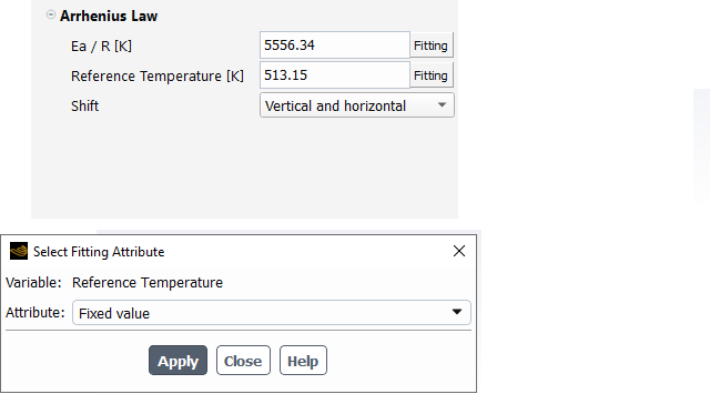
Once done, click . A similar procedure can be used to initialize a parameter to a specific value.
Repeat the previous three steps to define fixed values for any other parameters that you do not want changed during the fitting calculation.
For verification purposes, a summary of the parameters being fixed or (user-) initialized will be displayed in the Properties - Fitting panel. A typical example is shown below.
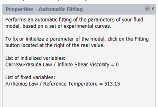
Within the context of the automatic fitting procedure in Fluent Materials Processing, you will need to read your experimental curve data directly into Fluent Materials Processing. Both .crv and .csv formats can be read.
To load an experimental curve, select:
![]() Rheometry →
Fitting → Experimental
Curves
Rheometry →
Fitting → Experimental
Curves ![]()
Alternatively, you can select ![]() Rheometry
→ Fitting → Experimental
Curves and press within the
Properties - Experimental Curves panel.
Rheometry
→ Fitting → Experimental
Curves and press within the
Properties - Experimental Curves panel.
In the Properties - Experimental Curves panel:
You enter a Name, which will be used for you to identify the curve in the data set.
Using under Filename, locate the experimental curve file and click to apply the file.
Specify the Curve Type of experimental curve. For a generalized Newtonian model, only steady shear viscosity curves can be loaded. For a viscoelastic fluid model, experimental curves can contain data on the steady shear viscosity, storage modulus G1 or loss modulus G2 vs angular frequency, transient extensional flow, or first normal stress difference N1 vs. shear rate.
Specify the corresponding temperature for thermal rheological fluid models under Temperature [K].
Note: If you plan to perform fitting for the temperature dependence of the rheological properties, you will need to supply several experimental data curves at different temperatures.
For the transient extensional flow, additional attributes need to be
specified. The mode can be uniaxial, biaxial or planar. The type of data can
be the viscosity vs time or the stress vs. (Hencky) strain  . The regime can be a constant extensional strain rate and
the corresponding strain rate is required, or constant extensional velocity
and the initial strain rate
. The regime can be a constant extensional strain rate and
the corresponding strain rate is required, or constant extensional velocity
and the initial strain rate  is required.
Repeat these steps if you have additional experimental curves to load.
To delete an experimental curve, right-click it in the Outline View and select .
You will need to set some parameters that will be used by Fluent Materials Processing when it calculates the curve(s) during the fitting process. To access the Fitting Parameters, select:
![]() Rheometry →
Fitting → Fitting
Parameters
Rheometry →
Fitting → Fitting
Parameters ![]()
In the Properties - Fitting Parameters panel, you can specify the range of shear rates and several other parameters, as described below. The list of Fitting Parameters depends on the selected model.
Maximum Number of Iterations
In general, 50 iterations (the default) are enough to get converged results. In some cases, more iterations are needed, especially for fitting viscoelastic models when large number of modes are involved.
Update Graphics After Each Fitting Run
This is activated by default and Ansys suggest to keep it unchanged. This allows you to check whether further improvements are reported after a new series of iterations.
Enable Fitting of Relaxation Times
By default, relaxation times are not fitted. Rather, they are distributed at a regular interval in the range specified (logarithmic scale) for the relaxation times (see below). However, it is possible to optimize the distribution of the relaxation times. This sometimes helps to obtain a better fit.
When activating the fitting of relaxation times, the range of relaxation times defined can be affected. The acceptable range of relaxation times is from (0.999*min_relax_time) to (1.001*max_relax_time). When this option is activated, the fitting can become more complex, requiring a few more iterations and increasing the calculation time to achieve a converged solution. By default, you do not fit the relaxation times.
Link Non-linear Parameters
When a multi-mode differential viscoelastic model is selected, all modes obey the same constitutive equation. Despite this, a multi-mode model may involve a long series of linear and non-linear parameters, which need to be identified on the basis of a few data only. You can activate the option to , so that parameters of a given type will be assigned the same value for all modes. This may improve the fitting procedure by increasing the sensitivity of the model properties with respect to parameters.
Relaxation Times Range
By default, relaxation times are not fitted but are distributed at regular intervals in the specified range (logarithmic scale). You can enter the values respectively in the boxes next to Relaxation Time Minimum and Relaxation Time Maximum.
Window of Shear Rates
If you want to compare rheological curves obtained for a steady shear flow, you will need to specify the minimum and maximum values of shear rate for the curves so that they will all be consistent. You can enter the values respectively in the boxes next to Shear Rate Minimum and Shear Rate Maximum [s^-1].
Window of Times
If you want to compare rheological curves obtained for a transient flow, you will need to specify the minimum and maximum values of time for the curves so that they will all be consistent. You can enter the values respectively in the boxes next to Time Minimum and Time Maximum [s]
Window of Angular Frequencies
If you want to compare rheological curves obtained for an oscillatory shear flow, you need to specify the minimum and maximum angular frequencies for the curves so that they are all consistent. You can enter the values respectively in the boxes next to Angular Frequency Minimum and Angular Frequency Maximum [rad/s]
Weight of the Shear Viscosity Curves
The weighting allows you to assign more importance to one or more curves compared to others. For example, in the fitting of a viscoelastic model, if you are not interested in fitting the shear viscosity, you could set the weighting for the shear viscosity curves to a much lower value than the others.
To set the weighting for the shear viscosity curves, enter the desired value in the box next to the item Shear Viscosity Curves. The default value is 1.
Weight of the Moduli G1 and G2 Curves
The weighting allows you to assign more importance to one or more curves compared to others. To set the weighting for the storage and loss moduli curves, enter the desired value under Moduli G1 and G2 Curves. The default value is 1.
Weight of the Extensional Viscosity Curves
The weighting allows you to assign more importance to one or more curves compared to others. For example, in the fitting of a viscoelastic model for a flow that is mainly extensional (fiber spinning), the fitting of the extensional viscosity must be better than the fitting of the other curves, so you should set the weighting for the extensional viscosity curves to a higher value than the others.
To set the weighting for the extensional viscosity curves, enter the desired value in Extensional Viscosity Curves. The default value is 1.
Weight of the First Normal Stress Difference N1 Curves
The weighting allows you to assign more importance to one or more curves compared to others. To set weighting for the first normal stress difference curves, enter the desired value in First Normal Stress Difference N1 Curves. The default value is 1..
To draw the experimental data curves in the chart, select:
![]() Rheometry →
Fitting → Experimental
Curves
Rheometry →
Fitting → Experimental
Curves ![]()
See Modifying Curve Display Attributes for information about changing the appearance of the curves.
When you have completed the setup of your fitting problem, begin the calculation by selecting:
![]() Rheometry →
Fitting
Rheometry →
Fitting![]() Run
Fitting
Run
Fitting
Fluent Materials Processing will automatically compute curves corresponding to all of the specified experimental data curves. When the automatic fitting calculation is complete, Fluent Materials Processing will save the results. You can export the rheological model to the setup at any time. See Exporting the Results of the Fitting.
Fluent Materials Processing will automatically update the chart with the computed curve(s) and the experimental curve(s). The steady shear viscosity, storage and loss moduli, and the first normal stress difference will be plotted on the same log-log graph. A second chart will display the extensional viscosity curve(s), using a linear scale for both the extensional viscosity and the time, unless otherwise specified. See Modifying Curve Display Attributes for information about changing the appearance of the curves.
If you want to plot curves other than those that were directly calculated,
you can select them by clicking ![]() Rheometry
→ Rheometric Curves and specifying the
required curves in the Properties - Rheometric Curves
panel.
Rheometry
→ Rheometric Curves and specifying the
required curves in the Properties - Rheometric Curves
panel.
In an automatic fitting for a viscoelastic model, steady shear viscosity, storage modulus, and loss modulus are the mandatory curves whereas, first normal stress difference and extensional viscosity are the optional curves. For a generalized Newtonian model, the steady shear viscosity is a mandatory curve. After an automatic fitting, it is possible to pursue fitting, if necessary.
Click ![]() Rheometry →
Fitting and select .
Rheometry →
Fitting and select .
This option is available when at least one fitting is complete. Fitting is
continued with the values of the parameters of the initialized model using
the values obtained at the previous fitting step. The fixed parameters will
not change. You do not have to change any flag associated to the parameter
under ![]() Setup →
Materials as Fluent Materials Processing automatically makes these
changes.
Setup →
Materials as Fluent Materials Processing automatically makes these
changes.
Calculations are stopped when the maximum number of iterations is reached, or if the following distances are adequately reduced:
The distance between two successive solutions.
The distances between the solution and the experimental points.
Given the assumption that a fluid model has n parameters to fit:
 | (4–110) |
If you compare the value of these parameters for two successive iterations i and i+1, respectively:
 | (4–111) |
 | (4–112) |
The distance  for parameter j
becomes:
for parameter j
becomes:
 | (4–113) |
where  = 10-6.
The global distance D is calculated as:
 | (4–114) |
In this case, assume you are comparing a single experimental curve to its calculated counterpart, at iteration i.
The experimental curve is composed of a set of P points:
 | (4–115) |
If  is the shear rate and if the shear rate range is
defined as
is the shear rate and if the shear rate range is
defined as  , the subset of points having
  in that interval is taken.
At iteration i, you can evaluate the model curve knowing the value of the parameters at that iteration:
 | (4–116) |
For the set of abscissas  , the model curve is composed of a set of
P points:
, the model curve is composed of a set of
P points:
 | (4–117) |
The distance  for point j can be defined
as:
for point j can be defined
as:
 | (4–118) |
such that
 | (4–119) |
Note: When there are several experimental curves, the distance printed in the listing will be the weighted sum of the distances of each curve.
Subsequently to an automatic fitting, you are encouraged to check the physical and numerical relevance of the calculated parameters. In addition, you always have the possibility to perform a subsequent manual parameter fitting.
Once the fitting completed, you can export the values for all the relevant
rheological parameters into the setup. This can be done by selecting
![]() Rheometry
Rheometry
![]() . The most recent values of the
parameters will be exported into the setup. From there it is then also
possible to export the complete material data into a file.
. The most recent values of the
parameters will be exported into the setup. From there it is then also
possible to export the complete material data into a file.
This chapter describes how to visualize the rheological properties of various fluid models and to fit them to experimental data, by defining or reading experimental data curves and plotting curves graphically using Fluent Materials Processing.
You can calculate property curves in Fluent Materials Processing or load .csv files previously created. For information about calculating and loading curves, see Rheological Properties and Working with Curves respectively. These curves are automatically displayed in the chart and become accessible when at least one curve is calculated. You can manipulate the display using your mouse and the various graphical user interface controls. Each curve can have different attributes (color, line). Curves that are calculated are saved in a sub-folder of the Fluent Materials Processing project folder.
When you click the button under the Properties - Rheometric Curves panel,
![]() Rheometry → Rheometric
Curves
Rheometry → Rheometric
Curves
The curves that were selected will be updated and added to the chart. This allows you to compare several models or fine tune a fitting. See Non-Automatic Fitting for details.
Note: You will not need to click and
Rheometry if you use
![]() Rheometry
→ Fitting as Fluent Materials Processing will automatically
update the chart for you after it completes the fitting calculation.
Rheometry
→ Fitting as Fluent Materials Processing will automatically
update the chart for you after it completes the fitting calculation.
The following terms are used throughout this chapter:
- axis
is a segment of a chart. Each axis has a range of values, and an interval (called a gap). You add a name to the axis, modify the format and precision of the printed numbers, and modify the range and the type of scaling (linear or logarithmic). See Modifying the Axis Attributes for details about modifying axis parameters.
- chart
is a window where curves are displayed. The chart is automatically created upon the first inquiry of a curve display. Multiple curves can be plotted on the same chart.
- curve
is a set of (x,y) pairs of values. The parameters of a curve include whether the data points are connected by a line, the color and thickness of the line, and the markers for the data points. See Working with Curves for information about selecting and modifying curves.
- plots
is a tab with a window where curves are displayed. Curve names are also listed next or under the chart. Right-clicking the Plots window provides access to the properties of axes, curves and charts.
This section describes the following topics:
The first format is .csv, and has the following structure:
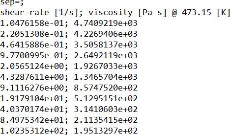
The first line displays the separator used, the second line is mainly
intended for you, the user, and the subsequent lines contain the data. It is
important that the last data line ends with
<CR>.
The second format is .crv, a legacy file format with the following structure:
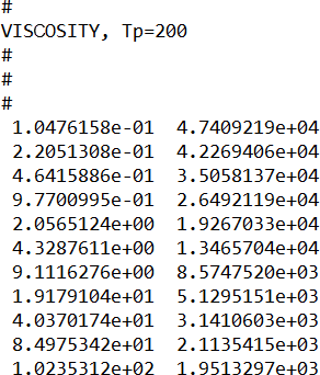
The first five lines do not contain any rheological data. Instead, the
second line contains useful information. The actual data is read from the
sixth line. Again, it is important that the last data line ends with
<CR>.
At least two data points are needed to draw a curve. Fluent Materials Processing can read files that contain many data points.
For information on reading curve files, see Reading Experimental Data Curves for the Automatic Fitting Method.
If you want to delete an experimental data curve, select the curve in
question under![]() Rheometry →
Fitting → Experimental
Curves and select . If you want to
delete a curve calculated by Fluent Materials Processing, unselect it from the list of
rheometric curves
Rheometry →
Fitting → Experimental
Curves and select . If you want to
delete a curve calculated by Fluent Materials Processing, unselect it from the list of
rheometric curves
![]() Rheometry → Rheometric
Curves
Rheometry → Rheometric
Curves
and click followed by .
Curves are automatically saved in a Rheometry subfolder located under C:\Users\myaccount\matpro-yyyy-mm-dd-hhmmss\Rheometry.
You can modify how a curve is displayed in the chart by selecting it in the curve list and using the curve settings.
To change the color of a curve, right-click the Plots window and select :
A dialog box opens where you can select the targeted curve:
Curves are identified by a title selected by Fluent Materials Processing, on the basis of your entered data for experimental curves, and on the basis of the selected rheometric curves for calculated properties. These types of curves are easily identified from each other via the letter 'x' or 'r' appearing at the beginning of the title, a letter respectively standing for experimental and rheometry.
When selecting a curve, a new dialog box opens where you can specify the color by selecting in the Basic colors section. You can choose to make a more general selection via the palette, the HSV/RGB values or via its HTML code.
Click . The chart is automatically updated.
To change the line of a curve, right-click the Plots window and select :
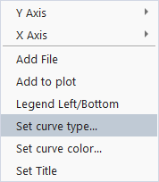
A dialog box opens where you can select the targeted curve:
Upon curve selection, a new dialog box opens where you can select the type of line:
Click . The chart is automatically updated.
Information about cleaning and modifying charts is presented in the following subsections.
A chart may contain many curves, resulting, for example, from the successive evaluation of model properties. To clean a chart:
Select
![]() Rheometry → Rheometric
Curves
Rheometry → Rheometric
Curves
in the Outline View and click in the Properties - Rheometric Curves panel, or
Select
![]() Fitting → Experimental
Curves
Fitting → Experimental
Curves
in the Outline View and click in the Properties - Experimental Curves panel.
Experimental curves will still be available for display, while rheometric curves corresponding to the most recent set of model parameters will be reevaluated upon request.
To modify the chart title, right-click the Plots window and select . Enter the title in the dialog box that opens and click .
Drawn curves are identified by a color and are accompanied by a legend. By default legends are displayed to the left of the chart. Legends can also be displayed below the chart. You can specify the location by right-clicking the Plots window and selecting .
There are several attributes of the axes that you can modify such as the range, the precision of the numbers attached to axis markers and the display of grids. All of these attributes are independently accessible for both vertical and horizontal axes (respectively Y- and X-axis) by right-clicking the Plots window.
To modify the range of values along the x-axis, right-click the Plots window, and select → .
A dialog box will open allowing you to specify the lower and upper bound of the X-axis, along with the syntax min, max:
The chart is automatically updated.
Right-click the Plots window and select to restore the calculated min and max values.
For changing the number of gridlines along the x-axis, right-click the Plots window and select → .
A dialog box opens where you can specify the number of gridlines:
The chart is automatically updated.
Note: The usual number of gridlines is 9 for a log scale.
To modify the precision of the numbers along the x-axis, right-click the Plots window and select → .
A dialog box opens where you can specify the precision along with the
syntax %.ne, where n indicates
the number of digits. For example %.1e if one digit
is required:
You can repeat the same operations for the y-axis by right-clicking the Plots window and selecting the . Two additional options will appear allowing you to select a linear or a log scale:
This section presents some guidelines for selecting an appropriate model and fitting the related parameters for several common applications.
- 4.11.5.1. Introduction
- 4.11.5.2. The Weissenberg Number
- 4.11.5.3. Viscometric and Rheometric Measurements
- 4.11.5.4. General Strategy for Fitting
- 4.11.5.5. Guidelines for Extrusion
- 4.11.5.6. Guidelines for Fiber Spinning
- 4.11.5.7. Guidelines for Film Casting
- 4.11.5.8. Guidelines for Blow Molding and Thermoforming
- 4.11.5.9. Guidelines for Pressing
- 4.11.5.10. Empirical Rules and Principles
There are several viscoelastic models available in Fluent Materials Processing, as described in Material Data Parameters. These models involve linear and nonlinear parameters, which in turn carry viscometric and extensional properties. It can often be a difficult task to select the best constitutive equation with the most appropriate material parameters. The task can be more easily addressed if it is broken into three smaller parts such as:
The number of modes.
Which constitutive equation are being used.
The parameter settings.
These parts implicitly assume that everything is known about the material being modeled and that all properties are equally important, which is usually not the case. Indeed, in actual industrial practice, only some of the information is known and assumptions are therefore necessary.
The purpose of this section is to suggest useful guidelines for the selection of a constitutive model and associated parameters. Two approaches are possible such as evaluating the numerical values of parameters to match some experimental data in a given range, or trying to fit all viscometric (and possibly elongational) measured data over a broad range. These two approaches lead more or less to the selection of a rheological model for a flow and to the selection of a rheological model for a fluid, respectively.
Although you may prefer one of these two approaches, useful guidelines can be found in both. Therefore, the guidelines that follow will be presented on the basis of the flow being simulated. For example, the kinematics involved in profile extrusion is significantly different from that in blow molding or thermoforming. Swelling during extrusion results from a velocity rearrangement and normal stress difference developed in a shear flow, while blow molding involves an elongational component with a strain-hardening or strain-thinning response from the melt.
Recommendations will be given for the four most-commonly encountered types of flow:
Extrusion (Guidelines for Extrusion).
Fiber spinning (Guidelines for Fiber Spinning).
Film casting (Guidelines for Film Casting).
Blow molding/thermoforming processes (Guidelines for Blow Molding and Thermoforming).
Consider a flow whose typical kinematics is given by  , and λ is the relaxation time of
the fluid. The Weissenberg number is given by
, and λ is the relaxation time of
the fluid. The Weissenberg number is given by
 | (4–120) |
This number indicates the elasticity involved in a flow.
The Weissenberg number is sometimes understood as the ratio between a normal-stress difference and a shear stress. Such an interpretation raises questions about the relevance of Weissenberg numbers as high as 20 or even 100. Indeed, this would involve a very high normal stress, and besides a few biological fluids, the majority of macromolecular fluids would not sustain such a high stress.
Important: Note that a polymer melt is characterized by a relaxation spectrum, rather
than by a single relaxation time. Hence, when evaluating  , it is important to consider an adequate relaxation time
λ.
, it is important to consider an adequate relaxation time
λ.
In general, you should obtain rheological measurements for the melt in the following order of importance: oscillatory properties (storage and loss moduli), steady-state shear viscosity, first normal-stress difference and/or transient uniaxial elongational viscosity. Of course, it is not always possible to obtain such an extensive range of measurements, which can often be costly.
This section describes the following topics:
The oscillatory properties (storage and loss moduli, represented by
 and
and  , respectively) should always be provided. For most polymer
melts, the measurement of the oscillatory properties is easy. Storage and
loss moduli are usually obtained over several decades. The most typical
measurement device is the cone-plate rheometer. Measurements can be taken at
one temperature if an isothermal model is being considered, or at various
temperatures if a thermal model is being considered.
, respectively) should always be provided. For most polymer
melts, the measurement of the oscillatory properties is easy. Storage and
loss moduli are usually obtained over several decades. The most typical
measurement device is the cone-plate rheometer. Measurements can be taken at
one temperature if an isothermal model is being considered, or at various
temperatures if a thermal model is being considered.
In general, measurements can be taken at various temperatures in order to
obtain master curves of  and
and  at a suitably selected temperature. For this, the
time-temperature equivalence can be used in order to properly shift the
curves. By doing so, it is possible to expand the range of experimental data
for the linear properties, provided that the material exhibits visible
temperature dependence. See Empirical Rules and Principles for details.
at a suitably selected temperature. For this, the
time-temperature equivalence can be used in order to properly shift the
curves. By doing so, it is possible to expand the range of experimental data
for the linear properties, provided that the material exhibits visible
temperature dependence. See Empirical Rules and Principles for details.
The steady-state shear viscosity is also always needed. When possible, it should also be measured using capillary rheometry, and the data for shear viscosity vs. true shear rate should be obtained. If such an experiment is not feasible, you can instead extract information about shear viscosity from the empirical Cox-Merz rule [4] , assuming that the modulus of the complex viscosity can be obtained from dynamic data. Alternatively, you can extract information about shear viscosity from the empirical mirror relationship of Gleissle [6], which suggests that the steady shear viscosity curve is a mirror image of the transient shear viscosity measured at a low shear rate. This assumes that transient viscosity measurements are indeed possible. See Empirical Rules and Principles for details.
Even though the knowledge of the shear viscosity is not important for all processes, the automatic fitting procedure requires it. Extrapolating from measured quantities can provide additional data, but data should not be extrapolated over more than one decade.
If available, the steady data of the first normal-stress difference is also useful. Data can be acquired using a cone-plate rheometer or using a technique based on the hole pressure. It is also possible to estimate the first normal-stress difference on the basis of capillary extrudate swell, by using an empirical formula suggested by Tanner [11].
If such data cannot be acquired, you can instead extract information about the steady first normal-stress difference using the empirical Cox-Merz rule [4] (p. 201), assuming that the storage modulus can reveal a good indication about the first normal-stress difference. See Empirical Rules and Principles for details.
Even though the knowledge of the first normal-stress difference is not important for all processes, the automatic fitting procedure can benefit from it. While extrapolating from measured quantities can provide additional data, data should not be extrapolated over more than one decade.
If available, transient uniaxial elongational viscosity data are also useful. Data should be obtained by measuring at a constant strain rate or constant stretching velocity, which can be accomplished using equipment involving the EVF technology or of the Münstedt type (for example, filament stretching).
This section describes the following topics:
- 4.11.5.4.1. Weighting Measured Data
- 4.11.5.4.2. Assigning a Value to a Parameter
- 4.11.5.4.3. Using Identical or Independent Nonlinear Parameters
- 4.11.5.4.4. Relaxation Time vs. Relaxation Spectrum in Extrusion, Fiber Spinning, and Film Casting
- 4.11.5.4.5. Relaxation Time vs. Relaxation Spectrum in Blow Molding and Thermoforming
- 4.11.5.4.6. Relaxation Time vs. Relaxation Spectrum in Pressing
Once you have obtained the data described in Viscometric and Rheometric Measurements, you can weigh their importance within Fluent Materials Processing, as described in Defining Numerical Parameters. This is useful if, for example, there is some uncertainty about the data for a particular property, or if some data have been measured at a different temperature.
Material parameters are specified within a range of acceptable values. For example, viscosity factors must be positive. If the automatic fitting method is used, each material parameter can have three types of status: subject to fitting, initial value, or fixed value. By default, all parameters are subject to fitting, meaning that Fluent Materials Processing will compute the best value based on the experimental data. If you have a priori knowledge of the value of a parameter, you can speed up the fitting calculation by assigning a fixed value to it.
Since there may be many parameters for a model, and there may be only a limited amount of experimental data available, it can be difficult to compute the best set of parameters. In this case, it is preferable to assign a fixed value to one or more parameters, so that they will not change during the fitting calculation.
If the model involves only one relaxation time, its value can be either assigned or computed by Fluent Materials Processing. For a multi-mode model, however, you will need to specify the spectrum of relaxation times yourself, or let it computed by Fluent Materials Processing. In that last case, you have just to specify the minimum and maximum possible relaxation times.
Next, there are nonlinear parameters for the models. For the PTT model
(described in Phan-Thien-Tanner Model), the parameters ε and
ξ control the elongational viscosity and
viscometric properties, respectively: an increasing
ε reduces or even cancels the strain hardening,
while ξ affects shear-thinning properties as well
as the amount of second normal-stress difference. Based on your needs,
knowledge, or available experimental data, you may want to fix these values.
Typically, strain hardening occurs for  to
to  , and disappears for
  . For example, low values for ε
should be specified for a LDPE, while moderate values are appropriate for a
LLDPE or a HDPE. On the other hand, shear thinning occurs for nonzero values
of ξ, which usually is set to about 0.2. For
practical purposes, it can be given a value of 0.5 or even as high as
1.
. For example, low values for ε
should be specified for a LDPE, while moderate values are appropriate for a
LLDPE or a HDPE. On the other hand, shear thinning occurs for nonzero values
of ξ, which usually is set to about 0.2. For
practical purposes, it can be given a value of 0.5 or even as high as
1.
The Giesekus model (described in Giesekus Model) involves the parameter α, which simultaneously increases shear thinning and the second normal-stress difference while it reduces the strain-hardening property. Again, based on your needs, knowledge, or available experimental data, you can fix the value of α. When viscometric properties are relevant for the flow, values of α ranging from 0.2 to 0.8 are common. If elongational properties are needed, α plays a role similar to ε in the PTT model, and very low values (10-3 to 10-2) should be considered if strain hardening is needed.
For a PTT model with a nonzero value of ξ or a Giesekus model with α>0.5, as well as for the DCPP and the Leonov models, in both single- and multi-mode models, it is important to check whether the shear stress remains a monotonically increasing function of shear rate. A non-increasing shear stress can be corrected by adding a purely Newtonian component to the stress tensor. For single mode PTT model with a zero value of ε and for single mode Giesekus model with α = 1, the viscosity of this component is at least 1/8 of the viscosity factor of the only mode. For single mode PTT model with a non-zero value of ε, for single mode Giesekus model with α less than 1, as well as for multi-mode models, the viscosity of this component can be lower.
The DCPP model (described in Differential Viscoelastic Models) involves the parameter ξ, which simultaneously increases shear thinning and the second normal-stress difference while the parameter q increases the strain-hardening property. You can fix the value of ξ and q, based on your requirements, knowledge, or available experimental data. When viscometric properties are relevant for the flow, values of ξ ranging around 0.2 are reasonable. If elongational properties are needed, and in particular if strain hardening is needed, the parameter q should be increased. It reflects the number of branches of the POM-POM macromolecule and therefore affects the behavior in elongation.
The Leonov model (described in Differential Viscoelastic Models) involves several nonlinear parameters, affecting
either the viscometric behavior or the elongation properties. You assign
values to some of these nonlinear parameters, based on your requirements,
knowledge, or available experimental data. Parameters q
and  affect the transition from trapped to free configuration
of macromolecular chains. When viscometric properties are relevant for the
flow, it is interesting to note that
affect the transition from trapped to free configuration
of macromolecular chains. When viscometric properties are relevant for the
flow, it is interesting to note that  enhances the shear thinning property, while
 increases the viscosity. Parameter
  has no effect on the shear viscosity, while it contributes
to a decrease of the elongational viscosity. If elongational properties are
needed it can be noted that increases the strain hardening, while and decrease it.
has no effect on the shear viscosity, while it contributes
to a decrease of the elongational viscosity. If elongational properties are
needed it can be noted that increases the strain hardening, while and decrease it.
It is possible that the fitting calculation yields values for nonlinear parameters that are unusual, although within the limits of accuracy. In this case, you should set these parameters to more appropriate fixed values, and rerun the fitting calculation. This will yield another set of parameters with the expected properties.
In general, the fitting calculation will determine parameter values on the basis of the available experimental data. However, the available data do not necessarily include the operating conditions, as measurement techniques do not always allow for reaching the conditions present in the actual process. Fiber spinning is a typical example, where the melt is processed at strain rates much higher than those available for rheometric measurement. For such cases, you can extrapolate from available data.
When a multi-mode differential viscoelastic model is selected, all modes obey the same constitutive equation. Despite this, a multi-mode model may involve a long series of linear and nonlinear parameters, which need to be identified based on some data only. You have the option of specifying that nonlinear parameters of a given type will be assigned the same value for all modes. This may sometimes improve the fitting procedure by increasing the sensitivity of the model properties with respect to nonlinear parameters.
Using identical values for nonlinear parameters of a given type is not a requirement; by default, the nonlinear parameters are independent. It is interesting to note that the time-temperature equivalence is advocated for using identical values for nonlinear parameters of a given type, although that argument does not formally hold for nonlinear properties. See Empirical Rules and Principles for details.
When a large amount of data is available, it can be tempting to build a
rheological model involving a broad relaxation spectrum, even ranging up to
100 s or beyond. In most cases, this will be impractical and not very
useful. Indeed, in a cessation of steady shear flow, measurements reveal
that the relaxation mechanism occurs with a time scale on the order of
 , where
  is a typical shear rate involved in the experiment.
This observation allows for the identification of a typical time scale for
the description of mechanisms occurring in steady flow processes, such as
extrusion, fiber spinning, or film casting. An extrusion flow is
characterized by a typical wall shear rate  , while fiber spinning and film casting are characterized
by a typical elongation rate
, while fiber spinning and film casting are characterized
by a typical elongation rate  . Consequently, if a single-mode constitutive equation is
selected, the corresponding relaxation time should be specified as about
. Consequently, if a single-mode constitutive equation is
selected, the corresponding relaxation time should be specified as about
 or
or  , respectively. For a multi-mode model, the relaxation
times should be selected in the vicinity of
, respectively. For a multi-mode model, the relaxation
times should be selected in the vicinity of  or
or  , respectively. This is quite important, since it enables
the setup of a model that is in agreement with the typical time scales
involved in the simulation. Note that the above comments also raise
questions about the relevance of Weissenberg numbers as high as 10 or 100.
, respectively. This is quite important, since it enables
the setup of a model that is in agreement with the typical time scales
involved in the simulation. Note that the above comments also raise
questions about the relevance of Weissenberg numbers as high as 10 or 100.
For most applications, the computational domain is open, with fluid entry and exit. The residence time of fluid particles in the computational domain usually remains moderate, so extremely long relaxation times are not usually effective. Fluid particles trapped in vortices usually do not affect the main flow; they are instead a consequence of it. Finally, in extrusion, the extruded material solidifies long before the effects of these long relaxation times become visible.
Typical time scales for blow molding and thermoforming are rather short: from on the order of a tenth of a second for a milk bottle, to on the order of a few seconds for a gas tank. Hence, starting from a reasonable assumed initial rest state, stresses develop within that time interval. Although the deformation speed (and therefore the strain rate) is usually unknown, deformations remain moderate. Consequently, dynamic or linear measurements alone provide a good characterization of the melt for blow molding and thermoforming.
The selected spectrum of the rheological model may, of course, involve very short times and very long times. Actually, very short time scales (that is, those smaller than the typical process time) can be replaced by a purely Newtonian contribution. Similarly, long times (that is, much longer than the process time) probably do not have the opportunity to develop their own contribution to the stresses, and can be omitted, if necessary.
Pressing applications are very similar to simple squeeze flows. Typical time scales for pressing applications are rather short: they range from on the order of a tenth of a second up to a few seconds. With the exception of rheometric measurements, they depend more or less on the geometrical size of the melt sample. Hence, starting from an initial rest state, stresses develop within that time interval. Although the rate of deformation can be large, deformations remain moderate. Consequently, dynamic or linear measurements alone provide a good characterization of the melt for pressing.
The selected spectrum of the rheological model may, of course, involve very short times and very long times. Actually, very short time scales (that is, those smaller than the typical process time) can be replaced by a purely Newtonian contribution. Similarly, long times (that is, much longer than the process time) probably do not have the opportunity to develop their own contribution to the stresses, and can be omitted if necessary.
Transient and steady-state situations can be considered for 2D viscoelastic extrusion simulations, while it is reasonable to essentially consider steady-state flow situations in 3D. Transient extrusion processes are encountered in parison production, while steady-state conditions are met for profile extrusion. The guidelines in this section focus on steady-state cases.
This section describes the following topics:
In 2D extrusion flows, swelling at the die exit is caused by both the velocity rearrangement and the relaxation of the normal stresses. The velocity profile in the channel results mainly from viscous forces, while the normal stress is a viscoelastic effect connected to the shear rate. The material may also exhibit properties such as strain thinning and strain hardening, but these effects in extrusion are negligible.
In 3D extrusion flows, the normal-stress difference also plays a role in the swelling, but velocity rearrangements in 3D generate much more dramatic effects than in 2D. Indeed, a 3D cross-section may be such that the resulting velocity distribution is strongly non-uniform. Typically, low velocities are encountered in narrow cross-sections and tiny details, while high velocities are encountered in wide-open regions. At the die exit,the local lack of flow rate, i.e. of extruded material, is responsible for significant deformations which develop in order to obtain a uniform velocity distribution in the extrudate. Quite obviously, this leads to a further reduction of the previously narrow cross-sections.
Therefore, more so in 3D than in 2D, an appropriate flow balancing inside the die (based on stresses, velocity, pressure, and so on) may improve the flow. Finally, as in 2D, the effects of the elongational properties are negligible, compared to those resulting from velocity rearrangement and normal-stress difference, and they can therefore be neglected.
The linear properties and nonlinear shear viscosity provide good insight into the viscoelastic character of the material being extruded. Also, if the nonlinear shear viscosity is not available, it can often be estimated using the Cox-Merz rule [4] or the Gleissle mirror relationship [6] (see Empirical Rules and Principles for details). When feasible, this set of experimental data can be usefully completed with first normal-stress difference data. For most materials, measurement of linear properties for angular frequencies ranging from 0.01 to 100 rad/s , or perhaps up to 1000 rad/s is achievable. If you consider a typical wall shear rate in the extrusion process, it is usually included within this range of measurements. Otherwise, extrapolation should be considered.
For 3D flows, it is practical to select a “computationally light"
rheological model, to reduce the computational cost of the
Fluent Materials Processing simulation. Hence, it is useful to identify a typical shear
rate  for the flow, and obtain viscometric data one decade on
each side of this shear rate. Doing this implicitly reinforces the idea of a
constitutive equation for a flow (rather than for a fluid). Consequently the
fitted model for a given shear-rate decade will probably not be the best one
for another shear-rate decade.
for the flow, and obtain viscometric data one decade on
each side of this shear rate. Doing this implicitly reinforces the idea of a
constitutive equation for a flow (rather than for a fluid). Consequently the
fitted model for a given shear-rate decade will probably not be the best one
for another shear-rate decade.
Consider the typical wall shear rate  in the extrusion process. If a constant viscosity is
observed around
in the extrusion process. If a constant viscosity is
observed around  , the Maxwell or Oldroyd-B model is recommended. If shear
thinning occurs around
, the Maxwell or Oldroyd-B model is recommended. If shear
thinning occurs around  , the PTT or Giesekus model is recommended. If qualitative
information on the macromolecular behavior is required, it can also be
interesting to consider using the DCPP model.
, the PTT or Giesekus model is recommended. If qualitative
information on the macromolecular behavior is required, it can also be
interesting to consider using the DCPP model.
For filled materials, such as rubber, the Leonov model can also be considered, but the large number of unknowns involved warns against having unrealistic modeling ambitions.
Both single- and multi-mode models are acceptable for a 2D model, but a single-mode model is strongly recommended for a 3D model.
For a single-mode model, select a relaxation time on the order of
 . For a two-mode model, select one relaxation time <
 and one >
  , with no more than one decade between relaxation times.
For a three-mode (or more) model, select relaxation times <
, with no more than one decade between relaxation times.
For a three-mode (or more) model, select relaxation times <
 and >
and >  , preferably with no more than one decade between
relaxation times.
, preferably with no more than one decade between
relaxation times.
For a strain-hardening material (for example, LDPE), a low value can be specified for the PTT model’s ε or the Giesekus model’s α. Values of 10-3 to 10-2 are typical. For strain-thinning or moderate strain-hardening materials (for example, LLDPE or HDPE), a higher value—typically about 0.1—can be specified. Also, for strain hardening materials, the DCPP model can be used with a large enough value of q (number of arms).
For the simulation of the flow of filled materials, the use of the Leonov model can be a good idea. The model involves several parameters, and have received reasonable default values. It is worth mentioning that the Leonov model involves the calculation of several tensors, and that the use of a multi-mode model can be computationally expensive.
Finally, for very large flow simulations, it may be relevant to consider the simplified viscoelastic model suggested in Simplified Viscoelastic Model, suited for extrusion simulation. Here, the identification of parameters is based on rheometric information, such as viscosity and swelling versus the flow rate. Typically, the first normal viscosity involved in the model equals the shear viscosity by default, while a relaxation time value or function and a weighting factor must be identified in order to reproduce the swelling behavior. That is, a 2D axisymmetric flow simulation is required for parameters identification.
In the automatic fitting procedure, it is preferable to consider the data in the range of shear rates of interest, typically one decade above and one below. If data extrapolation is necessary, it should be done over no more than one decade. Also, use appropriate weighting factors (see Weighting Measured Data) if some data are more reliable than others.
The whole shear viscosity curve for the model may differ from measurements at low shear rates, but this can generally be disregarded. Indeed, low shear rates are encountered only in a few areas of the flow, and involve usually a fraction of the total flow rate, such that the total impact on the momentum is negligible.
Transient and steady-state situations can be considered for 2D viscoelastic fiber-spinning simulations, while it is reasonable to essentially consider steady-state flow situations in 3D. Fiber spinning is a continuous process, so primarily steady-state simulations are relevant. The guidelines in this section will therefore focus on steady-state cases.
This section describes the following topics:
Several mechanisms are involved in 2D fiber spinning. First, a take-up velocity is assigned at the end of the computational domain. This velocity leads to significant geometric changes and to the development of the free surface. A swelling may develop at the die exit, but it is usually not a critical feature; it is quickly hindered or annihilated by the take-up (pulling) velocity.
The take-up velocity plays a dominant role in the free jet. A transverse velocity gradient exists in the die, while the free jet is endowed with an axial velocity gradient. The occurrence of a significant strain rate is typical for fiber spinning. Many melts involved in fiber spinning exhibit a more-or-less pronounced strain-hardening behavior, as this property is known to enhance the stability of the process.
A moderate take-up velocity is sometimes applied in continuous extrusion processes (for example, for guiding or stabilizing the extrudate). Here, the draw ratio is close to 1, which means that the elongation rate involved is often negligible; such cases should be regarded as extrusion instead of fiber spinning.
To some extent, 3D fiber spinning combines the effects encountered in 2D fiber spinning with some of those seen in 3D extrusion. That is, the flow has a strong elongational component due to the take-up velocity, and is affected by the velocity rearrangement in the 3D geometry. This take-up velocity leads to significant geometric changes. A swelling may develop at the die exit, but it is usually not a critical feature; it is quickly hindered or annihilated by the take-up (pulling) velocity.
The kinematics of 3D fiber spinning involves a transverse velocity gradient in the die, while the fiber itself is endowed with an axial velocity gradient. Consequently, the aspect ratio of some details in a cross-section of the fiber may differ significantly from the corresponding aspect ratio found at the die exit.
The elongational viscosity is important, perhaps even more so than the shear viscosity. This property can be measured for moderate strain rates (usually up to 10 s-1 using an elongational rheometer equipped with the EVF device), although the material is often processed at a much higher strain rate. This apparent difficulty can be overcome by considering the following heuristic argument. For a given melt, all curves of transient uniaxial elongational viscosity follow the same lower linear envelope, up to a Hencky strain of 1 or 2. It is therefore reasonable to believe that a similar behavior occurs at higher strain rates, regardless of whether the melt is strain-hardening or strain-thinning. This is a qualitative extrapolation, which results from a speculative extension of the Gleissle mirror relationship to the transient elongational viscosity.
The minimum experimental data needed for successful fitting are the linear properties and the nonlinear shear viscosity (possibly obtained from the Cox-Merz rule [4] or the Gleissle mirror relationship [6] (see Empirical Rules and Principles for details). If data for the transient elongational viscosity are available, they should also be used. When all the properties are available, you can allocate a low weighting to the shear viscosity and a high weighting to the elongational properties (as described in Defining Numerical Parameters), since the elongational component in the fiber is more important.
The PTT and Giesekus models recommended for extrusion are also recommended for fiber spinning. The Oldroyd-B and Maxwell models are also good choices, especially for highly strain-hardening materials. If qualitative information on the macromolecular behavior is required, it can also be interesting to consider using the DCPP model.
Both single- and multi-mode models are acceptable for a 2D model, but a single-mode model is strongly recommended for a 3D model. For a 2D model, three modes are recommended, with the relaxation times no more than one decade apart.
The flow involves a typical shear rate  in the die and a typical elongation rate
  in the fiber itself. Two or more orders of magnitude may
exist between these quantities. It is worth mentioning that the actual
deformation in shear evolves linearly with the shear rate, while the actual
deformation in elongation evolves exponentially with the elongation rate.
Therefore, although values for the typical shear rate in the die can be
larger than the values of the elongation rate in the fiber, the actual
corresponding deformation will be significantly larger in the fiber.
Consequently, you should focus on the elongation character more
carefully.
in the fiber itself. Two or more orders of magnitude may
exist between these quantities. It is worth mentioning that the actual
deformation in shear evolves linearly with the shear rate, while the actual
deformation in elongation evolves exponentially with the elongation rate.
Therefore, although values for the typical shear rate in the die can be
larger than the values of the elongation rate in the fiber, the actual
corresponding deformation will be significantly larger in the fiber.
Consequently, you should focus on the elongation character more
carefully.
For a single-mode model, select a relaxation time of about  . For a multi-mode model, select one relaxation time <
 and one >
  , preferably with no more than one decade between
relaxation times.
, preferably with no more than one decade between
relaxation times.
For a strongly strain-hardening material (for example, LDPE), use the Maxwell or Oldroyd-B model when the strain-rate is moderate. Otherwise, consider a low value of ε (typically 10-3 to 10-2) with the PTT model, or a low value of α with the Giesekus model (typically 10-3 to 10-2). For strain-thinning or moderate strain-hardening materials (for example, LLDPE or HDPE), use the PTT or Giesekus model with a higher value—typically about 0.1 or more—for ε or α. Also, for strain hardening materials, the DCPP model can be used with a large enough value of q (number of arms). Currently, the Leonov model and the “simplified viscoelastic model" are not recommended for fiber spinning simulations.
If data on elongational viscosity are available, they should be used for the fitting. If the resulting values of the fitting for the nonlinear parameters are not in agreement with the expected behavior of the melt, they can be fixed as noted in Assigning a Value to a Parameter.
In the automatic fitting procedure, it is preferable to consider the data in the range of angular frequencies and shear rates of interest, typically one decade below and one above. If data extrapolation is necessary, it should be done over no more than one decade. Also, use appropriate weighting factors (see Weighting Measured Data) if some data are more reliable than others.
The shear viscosity curve for the model may differ from measurements, but this can generally be disregarded, since elongation is the main component of the flow.
This section describes the following topics:
Film casting processes exhibit features that are very similar to those encountered in fiber spinning (described in Guidelines for Fiber Spinning). That is, the extension results from a take-up velocity, which is significantly higher than the velocity at the die exit. An appropriate modeling approach for film casting in Fluent Materials Processing involves the use of a flat membrane element. Such an approach focuses on the development of the extruded film only, not on the flow inside the die.
Elongation is the component that dominates the flow, and a proper description of the elongational behavior of the material is needed, although draw ratios are usually lower than in fiber spinning. The comments about experimental data for fiber spinning are valid for film casting as well.
The PTT and Giesekus models recommended for fiber spinning are also recommended for film casting. The Oldroyd-B model is another acceptable choice, especially for melts characterized by a significant strain hardening behavior. The DCPP model can also be used, especially if a qualitative description of the macromolecular behavior is required. The Leonov model, however, is not available for film casting applications. In addition, the simplified viscoelastic model is not suited for the simulation of film casting.
If no experimental data are available for the elongational viscosity, the
nonlinear parameters should be fixed on the basis of known melt properties.
Therefore, for a strain-thinning or weakly strain-hardening melt, high
values for the nonlinear parameters are selected (typically  for a PTT model or
  for a Giesekus model). For a strain-hardening melt, lower
values should be used for the nonlinear parameters. If the DCPP model is
used, a relatively large number of branches (
for a Giesekus model). For a strain-hardening melt, lower
values should be used for the nonlinear parameters. If the DCPP model is
used, a relatively large number of branches ( in Equation 4–62) should be considered
for strain-hardening materials such as LDPE, while a unit or low number of
branches should be selected for strain-thinning or weakly strain-hardening
melts such as LLDPE.
in Equation 4–62) should be considered
for strain-hardening materials such as LDPE, while a unit or low number of
branches should be selected for strain-thinning or weakly strain-hardening
melts such as LLDPE.
Any prediction of blow molding or thermoforming is based on a transient calculation. The melt undergoes deformations in time, and the process conditions (such as the closing speed of the mold and the inflation pressure) may also vary with time.
In 2D, an axisymmetric geometry is often used in the Fluent Materials Processing calculation, although a planar description can also be used. Such a representation enables calculation through the thickness, and therefore prediction of the possible local shear effects. This is also the case when running an actual 3D calculation. For thin 3D objects in 3D, a membrane element is used, since it allows for calculation of complex shapes at a moderate cost. This representation is suited for elongation-like deformations but is unable to report shear deformations across the thickness.
This section describes the following topics:
In blow molding and thermoforming, extension is the dominating component of the deformation. Extension develops in two main directions, and is accompanied by a reduction in thickness. The magnitudes of the extensions in the main directions may differ, and they depend on the geometry. For example, inflating a cylinder involves an azimuthal extension field, while inflating a sphere involves an isotropic extension field.
Since extension is the main component in this process, knowledge of the extensional response of the material is usually necessary. However, although the extension rates can be high, the overall deformation often remains moderate. The Hencky strains are typically on the order of 1 or 2, which correspond to Cauchy strains up to 7.
Since the processes involve important strain rates and moderate extensions, knowledge of the transient linear extensional response is enough for the description of the melt rheology. That is, knowledge of the linear properties is a good starting point. If extensional data are available, they can be used (either in the automatic fitting calculation, or for checking the results of the automatic fitting). The extensional viscosity can be measured for moderate strain rates (usually up to 10 s-1 using an elongational rheometer equipped with the EVF device), although the material can be processed at a higher strain rate.
Although shear is usually not an important component of the total deformation, shear viscosity is needed in the fitting procedure. This can be obtained from the Cox-Merz rule [4] (see Empirical Rules and Principles), and can be assigned a zero weight (see Weighting Measured Data).
Several modeling approaches can be considered. The constant-viscosity Newtonian model is the simplest approach, and this is recommended if no rheological data are available. The use of a (shear-thinning) generalized Newtonian fluid model should not be considered for blow molding or thermoforming, since such a model will lead to unrealistically high velocities due to strain thinning.
Further modeling recommendations for 2D and 3D simulations are provided below.
In addition to the constant-viscosity Newtonian model, differential viscoelastic models (Maxwell, Oldroyd-B, PTT, Giesekus, FENE-P, DCPP, and Leonov) are available for blow molding and thermoforming. Although multi-mode simulations are available, for reasons of computational cost in Fluent Materials Processing, single-mode transient viscoelastic calculations are suggested, at least in first instance.
The flow involves a typical time scale τ, corresponding to the inflation time. The relaxation time should be of the same order of magnitude as this time scale.
For the viscosity factor, select a value corresponding to the shear viscosity as obtained for a shear rate of 1/τ.
For a strongly strain-hardening material (for example, LDPE), you can use the Maxwell or Oldroyd-B model when the strain rate remains moderate. Alternatively, you can use a low value of ε (typically 10–3 to 10–2) with the PTT model, a low value of α with the Giesekus model (typically 10–3 to 10–2), or a high value of q for the DCPP model. For strain-thinning or moderate strain-hardening materials (for example, LLDPE or HDPE), use the PTT or Giesekus model with a higher value—typically about 0.1 or more respectively for ε or α or the DCPP model with a low value of q.
If data on elongational viscosity are available, they should be used for the fitting. If the resulting values of the fitting for the nonlinear parameters are not in agreement with the expected behavior of the melt, they can be fixed as noted in Assigning a Value to a Parameter.
In the automatic fitting procedure, it is preferable to consider the data in the range of angular frequencies and deformation rates of interest, typically one decade above and one below the value 1/τ. If data extrapolation is necessary, it should be done over no more than one decade. Also, use appropriate weighting factors (see Weighting Measured Data) if some data are more reliable than others.
A purely Newtonian contribution can be added to the model. This corresponds to that part of the spectrum associated with very short times, and the response of which is shorter than the process time τ itself.
The shear viscosity curve for the model may differ from measurements, but this can generally be disregarded, since elongation is the main component of the flow.
For computational reasons, the use of the shell element (membrane element) is recommended for blow molding or thermoforming simulations that involve objects that are thin and have geometrically complex shapes. In addition to the constant-viscosity Newtonian model, the integral viscoelastic KBKZ model with a relaxation spectrum is also a good choice since a Lagrangian representation is used. No damping is considered due to the moderate deformations involved in the process, and the model reduces to the Lodge-Maxwell equation. The Lodge-Maxwell model predicts strain hardening up to a level that is experimentally observed.
Based on the oscillatory properties, a spectrum of 4 to 8 relaxation times is recommended. If you use a low number of relaxation times, they should be selected around the typical process (inflation) time τ. If you use a high number of relaxation times, they can spread to values as short as 10–4 and as long as 104 s.
Oscillatory data should be considered in the range of angular frequencies as covered by the range of reciprocal relaxation times. Viscosity factors should be identified based on linear oscillatory properties and shear viscosity as needed by the fitting tool in Fluent Materials Processing. A very low weighting can be used for the shear viscosity. If available, data on alongational viscosity should be used.
A purely Newtonian contribution can be added to the model. This corresponds to that part of the spectrum associated with very short times, and the response of which is shorter than the process time τ itself.
The shear viscosity curve for the model may differ from measurements, but this can generally be disregarded, since elongation is the main component of the flow.
Any prediction of pressing is based on a transient calculation. The melt undergoes deformations in time in the same manner as a simple squeeze flow. The process conditions (such as mold or plug motion) may also vary with time.
In terms of geometry, 2D planar, axisymmetric, and 3D modeling can be employed in the Fluent Materials Processing calculation. Such a representation enables a calculation through the thickness, and therefore it is possible to predict the local shear effects, as well as the elongation effects. For the former, 2D modeling can certainly make sense from a computational point of view.
This section describes the following topics:
In pressing, shear is the dominating component of the deformation, but it is often accompanied by a significant level of extension. The balance between shear and extension depends on the geometry, as well as on the boundary conditions. For example, shear will often dominate under the adhesion condition, while elongation may play a significant role under full slipping.
Since shear is often the main deformation component that develops in this process, knowledge of the shear viscosity of the material is necessary. While shear rates can be high, the overall deformation usually remains moderate. A Cauchy strain of the order of ten is a reasonable order of magnitude.
Since the processes are so affected by shear rates, obtaining information about the shear viscosity is the first step. Data acquisition via a direct capillary measurement is a good idea, although other techniques are acceptable. Linear properties and elongation data can also be used (either in the automatic fitting calculation or for checking the results of the automatic fitting), if they are available.
The extensional viscosity can be measured for moderate strain rates, usually up to 10 s-1 using an elongational rheometer equipped with the Extensional Viscosity Fixture (EVF).
As a first comment, it is worth noting that kinematic constraints imposed in the process do not really enable a full development of viscoelastic effects.
Several modeling approaches can be considered. The constant-viscosity Newtonian and generalized Newtonian models are the simplest approaches, and these are recommended when only the viscosity data is available. The generalized Newtonian fluid model is an obvious choice, because shear is an important component of the flow.
In addition to the Newtonian and generalized Newtonian models, differential viscoelastic models (Maxwell, Oldroyd-B, PTT, Giesekus, FENE-P, DCPP, and Leonov) are all good candidates for pressing simulations. Although multi-mode simulations are available, single mode transient viscoelastic calculations are recommended (at least in first instance) because of the computational cost in Fluent Materials Processing.
The flow involves a typical time scale  corresponding to the pressing. The relaxation time should
be of the same order of magnitude as this time scale. For the viscosity
factor, select a value corresponding to the shear viscosity, as obtained for
a shear rate
corresponding to the pressing. The relaxation time should
be of the same order of magnitude as this time scale. For the viscosity
factor, select a value corresponding to the shear viscosity, as obtained for
a shear rate  that is typical for the process.
For a strongly strain-hardening material (for example, LDPE), you can use
the Maxwell or Oldroyd-B model, as long as the strain rate remains
relatively low and therefore prevents the development of high stresses.
Alternatively, if you use the PTT or the Giesekus model, you should consider
specifying a low value for  or
or  , respectively: typically, between
10-3 to 10-2. You can
also use the DCPP model with a large number of branches (
, respectively: typically, between
10-3 to 10-2. You can
also use the DCPP model with a large number of branches ( ). For filled materials, the Leonov model could be
recommended, although it is computationally expensive.
). For filled materials, the Leonov model could be
recommended, although it is computationally expensive.
You can use data on the elongational viscosity if it is available. If the resulting values for the nonlinear parameters are not in agreement with the expected behavior of the melt, they can be fixed as noted in Assigning a Value to a Parameter.
It is often helpful during fitting to be able to estimate property values when experimental data is unavailable. For some materials, there are rules that link properties together; such rules are often empirical and must be handled with care, as there is no theoretical proof that validates their results. Frequently, these rules are applicable to polymer melts, such as polyethylenes and polystyrenes.
For information about some empirical rules and principles, see the following sections:
For many materials, linear data  and
and  is relatively easy to measure for various angular
frequencies
is relatively easy to measure for various angular
frequencies  (rad/s). When applicable, the shear viscosity can be
estimated by applying the Cox-Merz [4] empirical
rule. This empirical rule states that the modulus of the complex viscosity
matches the nonlinear shear viscosity, as shown in the following
equation.
(rad/s). When applicable, the shear viscosity can be
estimated by applying the Cox-Merz [4] empirical
rule. This empirical rule states that the modulus of the complex viscosity
matches the nonlinear shear viscosity, as shown in the following
equation.
 | (4–121) |
A Cox-Merz rule also exists for the first normal stress difference; it is an approximation for low shear rates and is written as follows:
 | (4–122) |
When performing a shear startup experiment for several values of the shear
rate, you measure the shear stress as a function of time; the transient
shear viscosity is obtained as the ratio of the shear stress and the
(constant) shear rate. In general, the measured curves exhibit an initial
development of the transient viscosity that matches the linear behavior
 , and subsequently departs from the linear response. The
departure from the linear response is delayed when a low shear rate is
considered.
, and subsequently departs from the linear response. The
departure from the linear response is delayed when a low shear rate is
considered.
The Gleissle mirror relationship [6] is
empirical and relates the linear transient viscosity,  with the nonlinear steady shear viscosity,
  as follows:
 | (4–123) |
There is a graphical mirror relationship between the transient shear viscosity and the nonlinear steady shear viscosity. This relationship has been observed for oils, as well as polymeric melts such as polyisobutylenes and polyethylenes. It also provides a useful tool for validating measurements obtained via various techniques.
A second Gleissle mirror relationship concerns the first normal stress
coefficient,  . It is given by:
 | (4–124) |
Again, there is a graphical mirror relationship between the transient first normal stress coefficient and the corresponding nonlinear steady property.
When necessary, it may be possible to extend the Gleissle mirror relationship for obtaining preliminary information on the transient elongation viscosity.
 | (4–125) |
The Cox-Merz rule for the first normal stress difference is only valid for a limited range of shear rates. Laun [7] has proposed an empirical rule that is valid over a larger interval of shear rates, and is given by the following:
 | (4–126) |
Equation 4–126 is found to be valid for polyethylenes. Similar relationships can be created for other families of polymers.
Using an elastic recoil mechanism, Tanner [11] proposed a simple expression that relates the extrudate diameter to the first normal stress difference, as follows:
 | (4–127) |
where  and
and  are the diameters of the extrudate and of the die,
respectively, and
are the diameters of the extrudate and of the die,
respectively, and  is the wall shear stress in the capillary die.
Time-temperature equivalence (or superposition) can be
applied, for example, in the measurements of linear properties
 and
and  . Usually, devices allow a measurement within a given
interval of angular frequencies. However, when performing measurements at
different temperatures, it is possible to expand the interval of angular
frequencies. If the relationship between linear properties and temperature
is unknown, it is reasonable to assume that the dependence is the same for
. Usually, devices allow a measurement within a given
interval of angular frequencies. However, when performing measurements at
different temperatures, it is possible to expand the interval of angular
frequencies. If the relationship between linear properties and temperature
is unknown, it is reasonable to assume that the dependence is the same for
 and
and  . Therefore, the ratio
  , when plotted against the angular frequency, will
typically have the same shape for different temperatures, though the curves
will shift along the horizontal axis. That is, an experiment performed at a
lower temperature corresponds to an experiment at a higher temperature
within a higher interval of angular frequencies. You can then combine the
data by shifting the curves and thereby expand the interval of angular
frequencies, possibly beyond the technological limits of the measurement
device. Simultaneously, the identification of the corresponding shift factor
will characterize the dependence with respect to temperature for subsequent
analysis; this is relevant, for example, for the complex viscosity. It is
therefore possible to acquire information on the temperature dependence of
the properties, as well as to expand the knowledge of linear
properties.
, when plotted against the angular frequency, will
typically have the same shape for different temperatures, though the curves
will shift along the horizontal axis. That is, an experiment performed at a
lower temperature corresponds to an experiment at a higher temperature
within a higher interval of angular frequencies. You can then combine the
data by shifting the curves and thereby expand the interval of angular
frequencies, possibly beyond the technological limits of the measurement
device. Simultaneously, the identification of the corresponding shift factor
will characterize the dependence with respect to temperature for subsequent
analysis; this is relevant, for example, for the complex viscosity. It is
therefore possible to acquire information on the temperature dependence of
the properties, as well as to expand the knowledge of linear
properties.
To illustrate how time-temperature equivalence can be
used, consider the following figure, which shows the measurement of linear
properties  (thick lines) and
  (thin lines) for angular frequencies ranging from
10–2 to 102.
The data is measured at four temperatures, represented here in black, blue,
magenta, and red.
(thin lines) for angular frequencies ranging from
10–2 to 102.
The data is measured at four temperatures, represented here in black, blue,
magenta, and red.
![G' and G" vs. Angular Frequency [rad/s]](graphics/g_pm_sec_guidelines_FigA__g1_g2.png)
The next figure shows the properties  , for each temperature ranging from black to red. The blue
temperature is the reference temperature that will be used to build the
master curves.
, for each temperature ranging from black to red. The blue
temperature is the reference temperature that will be used to build the
master curves.
![G"/G' vs. Angular Frequency [rad/s]](graphics/g_pm_sec_guidelines_FigB__tan_d.png)
The curves from the previous figure can be combined into a single curve, as shown in the following figure. The black curve is shifted to the right, while the magenta and red curves are shifted to the left; the shift factors are kept for further evaluation of the temperature dependence of the properties. Combining these four curves into the dashed line enables you to expand the interval of angular frequencies.
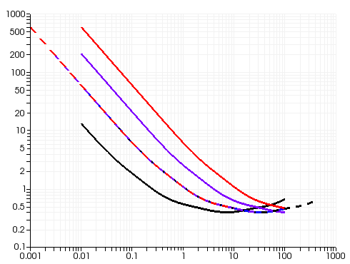
The shift factors obtained in the previous step can be applied to the
linear properties  and
and  , in order to obtain the master curves in the figure that
follows.
, in order to obtain the master curves in the figure that
follows.
![Master Curves for G' and G" vs. Angular Frequency [rad/s]](graphics/g_pm_sec_guidelines_FigD__g1_g2_shift.png)
The applicability of the time-temperature equivalence depends on the material considered, and is affected by the actual temperature dependence of the properties. Experience and specialized literature can provide further information.