


The best way to determine the quality of a mesh is by looking at statistics such as maximum skewness, rather than just performing a visual inspection. Unlike structured meshes, unstructured meshes are nearly impossible to comprehend with only a graphical plot. The Mesh category of the ribbon (Performing Meshing Diagnostics and the menu has a variety of reporting capabilities. The types of mesh information that can be reported include:
The size, quality, and statistics of a mesh, minimum, maximum, and average values of cell/face size and quality along with summary reporting and investigative tools for studying and trouble-shooting the mesh in fine detail. See Performing Meshing Diagnostics for details.
The size of the mesh (that is, the number of nodes, faces, and cells in it): use the Report Mesh Size dialog box.
>
Minimum, maximum, and average values of face size and quality: use the Report Face Limits dialog box.
>
Minimum, maximum, and average values of cell size and quality in a volume mesh: use the Report Cell Limits dialog box. The default quality measure is skewness, but you can also report the limits based on other quality measures or the range of change in cell size.
>
Boundary cell quality limits: use the Report Boundary Cell Limits dialog box.
>
Information about individual components of the mesh: use the
print-infocommand.
Important: If you used domains to generate the mesh or group zones for reporting (as described in Using Domains to Group and Mesh Boundary Faces), the report will apply only to the active domain.
These diagnostics and reporting operations are described in the following sections.
While Fluent Meshing already contains a number of separate mesh diagnostic tools, the Mesh category in the Ribbon includes many useful mesh checking and quality diagnostics from a single access point.

Note: You can also perform mesh diagnostics using the text user interface. See diagnostics/ for more information.
Use the Mesh > Check Ribbon menu to access common mesh checking and diagnostic commands.
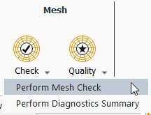
Perform Mesh Check: checks the mesh statistics and prints details to the console window. For example:
----------------------------------------
Mesh Check Scope   : 1 Objects, 14 Face Zones, 2 Cell Zones
Objects            : (manifold-solid_up)
----------------------------------------
Domain extents.
  x-coordinate: min = -3.627150e+02, max = 1.345893e+01.
  y-coordinate: min = -1.250188e+02, max = 2.475194e-09.
  z-coordinate: min = -1.018232e+02, max = 1.343616e+01.
Volume statistics.
  minimum volume: 3.402263e-05.
  maximum volume: 2.673741e+02.
    total volume: 1.512242e+06.
Face area statistics.
   minimum face area: 7.036576e-03.
   maximum face area: 3.314637e+01.
   average face area: 2.873890e+00.
Checking number of nodes per edge.
Checking number of nodes per face.
Checking number of nodes per cell.
Checking number of faces/neighbors per cell.
Checking cell faces/neighbors.
Checking isolated cells.
Checking face handedness.
Checking periodic face pairs.
Checking face children.
Checking face zone boundary conditions.
Checking for invalid node coordinates.
Checking poly cells.
Checking zones.
Checking neighborhood.
Checking interfaces.
Checking modified centroid.
Checking non-positive or too small area.
Done.
----------------------------------------
By default, the extent, or scope, of the mesh check depends on the current state of the workflow. The scope can include all or some of the existing objects (for example, geometry objects, meshing objects, and unreferenced objects). Use the Diagnostics Scope dialog box to change the scope of the analysis (see Setting the Scope of Your Diagnostics).
Perform Diagnostics Summary: diagnoses the mesh and prints a summary to the console window. The summary can contain surface and volume statistics, as well as recommendations for further analysis. For instance:
----------------------------------------
Diagnostics Scope  : 1 Objects, 22 Face Zones, 5 Cell Zones
Objects            : (hemisphere_mb)
----------------------------------------
Surface Diagnostics :

Total Number of Faces          =     4040
Maximum Skewness               =     0.28
Maximum Aspect Ratio           =    15.53
Number of Free Faces           =        0
Number of Multi Faces          =      982 --> found on 22 face zone(s)
Number of Self Intersections   =        0
Number of Cross Intersections  =     1290 --> found on 8 face zone(s)
Number of Self Proximity       =        0
Number of Point Contacts       =        0
Number of Invalid Normals      =        0
----------------------------------------
Volume Diagnostics :

Total Number of Cells          =    18374
Minimum Orthogonal Quality     =     0.19
Maximum Aspect Ratio           =    21.79
-----------------------------------------
By default, the extent, or scope, of the summary depends on the current state of the workflow. Along with surface and volume statistics, the summary can include any unreferenced cell zone ids and their associated face zone ids. Use the Diagnostics Scope dialog box to change the scope of the analysis (see Setting the Scope of Your Diagnostics). .
Use the Mesh > Quality Ribbon menu to access common mesh quality evaluations and tools.
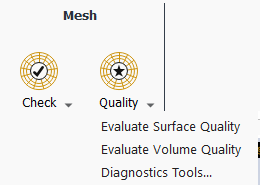
Evaluate Surface Quality: performs a surface quality evaluation and prints a summary to the console window. For instance:
----------------------------------------
Surface Quality [Measure : Skewness]
Minimum = 2.2357664e-06, Maximum = 0.56028138, Average = 0.036612933.

Marking Face in Range (0.51028138 0.56028138)...
--------------- ----------
 Cluster Number Entity Count
--------------- ----------
              1          1
              2          1
This command also automatically displays poor-quality marked faces in the graphics window.
Note: Certain surface diagnostics, such as checks for free surfaces, multiple faces, self intersections, and so on, are not supported in parallel, when the mesh is distributed. Surface mesh diagnostics are only necessary prior to generating a volume mesh (where the mesh is distributed). Once you generate a volume mesh, surface diagnostics are not required (and the Evaluate Surface Quality option will be grayed out and unavailable).. If a surface mesh is subsequently required, you can always agglomerate the mesh, or save the mesh and read it back into Fluent Meshing.
Evaluate Volume Quality: performs a volume quality evaluation and prints a summary to the console window. For instance:
----------------------------------------
Cell Quality [Measure : Orthogonal]
Minimum = 0.25625551, Maximum = 0.97745704, Average = 0.73252959.

Marking Cells in Range (0.25625551 0.30625551)...
--------------- ----------
 Cluster Number Entity Count
--------------- ----------
              1          2
              2          1
This command also automatically displays poor-quality marked cells and the specific region in the graphics window.
Diagnostic Tools...: opens the Diagnostics Tools dialog box (see Using the Diagnostics Tools Dialog Box).
The Diagnostics Tools dialog box provides access to several diagnostic resources in a single tool.
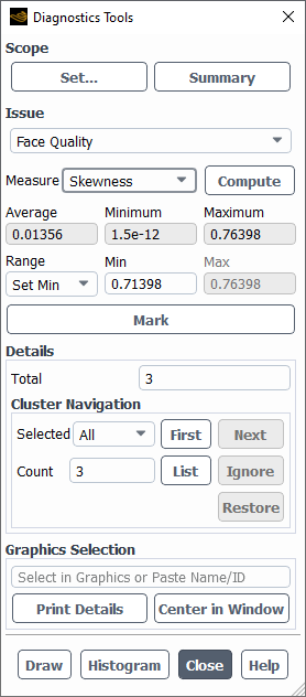
From this tool, you have convenient access to the following:
Use the Scope fields to control the scope and breadth and focus of the diagnosis for the current mesh.
Click the Set... button to open the Diagnostics Scope dialog box where you can change the scope of the analysis (see Setting the Scope of Your Diagnostics).
Click the Summary button to print a general diagnosis summary of the loaded mesh to the console window. The summary includes information about regions (names and number of face/cell zones), face/cell zone summaries, surface and volume checking and diagnostics reporting, suggestions for further diagnostics, and so on. The summary is based on whatever specific scope settings have been applied using the Diagnostics Scope dialog box. For example:
----------------------------------------
Diagnostics Scope  : 1 Objects, 13 Face Zones, 1 Cell Zones
Objects            : (multizone_prism_3zones)
----------------------------------------
Surface Diagnostics :

Total Number of Faces          =     4468
Maximum Skewness               =     0.56
Maximum Aspect Ratio           =     1.88
Number of Free Faces           =       52 --> found on 4 face zone(s)
Number of Multi Faces          =      312 --> found on 8 face zone(s)
Number of Self Intersections   =     1431 --> found on 6 face zone(s)
Number of Cross Intersections  =     1290 --> found on 8 face zone(s)
Number of Self Proximity       =     1349 --> found on 2 face zone(s)
Number of Point Contacts       =        0
Number of Invalid Normals      =        0
----------------------------------------
Volume Diagnostics :

Total Number of Cells          =     3851
Minimum Orthogonal Quality     =     0.26
Maximum Aspect Ratio           =     2.72
Number of Isolated Cells       =        0
----------------------------------------
Use the Issues fields to investigate problematic areas of your mesh, based on the summary. Issues can be categorized by Face Quality, Free Faces, Multi Faces, Self Intersections, Cross Intersections, Self Proximity, Point Contacts, Invalid Normals, Cell Quality, Stair-Step Locations, Isolated Cells,Exposed Quads, Modified Centroid, and Domain Extents.
Note: Any identified isolated cells will be listed in the diagnostic summary and when marked, can be removed using the Delete button.
Note: Based on the results of using the Summary button, only the problematic Issues and the Domain Extents will be available to diagnose. So if the overall summary lists no free faces or self intersections in the entire mesh, for example, then there is no need to diagnose them.
When the Issue is set to Face Quality or Cell Quality (when applicable), use the Measure field to further investigate mesh issues based on mesh quality measures.
Face quality measures include Skewness, Area, Size Change, Aspect Ratio, and Dihedral Angle.
Cell quality measures include Orthogonal, Skewness, Volume, Size Change, Aspect Ratio, and ICEMCFD.
For a selected cell/face quality measure, click the Compute button to calculate the Average, Minimum, Maximum cell/face values. A histogram is generated for the whole range by default. Vary the Min and Max as needed using the Range drop-down. You can change the Range to be set manually in a specific range of values (In Range), or to set the upper limit (Set Max), or to set the lower limit (Set Min). The default settings are adjusted accordingly based on the selected Measure.
When the Issue is set to Domain Extents, you are presented with the x, y, and z minimum and maximum values for a bounding box that defines the extents of the mesh domain (Xmin, Ymin, Zmin, Xmax, Ymax, and Zmax).
To inspect a particular portion of your mesh, enable the Update Bounds on Selection check box and select a face or zone in the graphics window (or enter specific values for the x, y, or z min/max fields). This will change the extents of the domain according to what you have selected in the graphics window or the fields, and display a specific portion of your mesh. To return to the original bounding box values, disable the check box and click the Compute button.
Note: The Domain Extents controls can also be used in conjunction with the Graphical Selection fields, where you can print out details of the selected objects in the console window, and center the selected object in the graphics window.
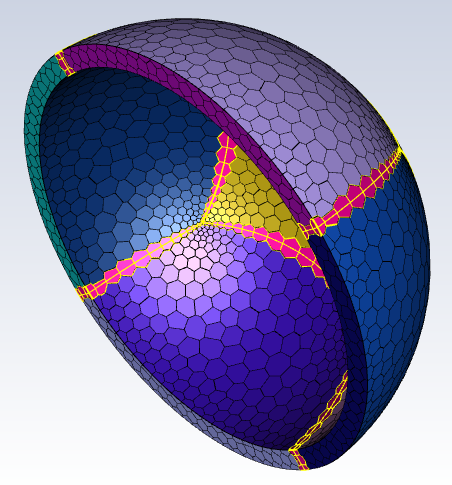
When applicable, use the Mark button to visibly mark problematic facets and isolate and automatically visualize all or portions of your mesh in the graphics window, based on the selected Issue (excluding Domain Extents). Collections of problematic facets are grouped into clusters that you can examine separately.
Note: Though generally performed automatically when using the meshing diagnostics tools, keep in mind that you can always use the Mark Faces check box in the Display category in the Ribbon to show/hide marked faces.
Use the Details fields to investigate your marked clusters and navigate through them to further identify any problems in your mesh. The Total field indicates the total number of clusters of marked cells. The Cluster Navigation fields let you view some or all of the identified clusters.
Use the Selected drop down list to select a particular cluster, or to select All of them (the graphics window will display the current selection). Alternatively, you can use the First and Next/Previous buttons to navigate through the collection of clusters as well. As you navigate your clusters, they are individually displayed in the graphics window for closer examination. If an identified cluster is acceptable and presents no problems, use the Ignore button to remove it from the list of problematic clusters (and use the Restore button to re-add any ignored clusters).
Use the Count to identify the number of problematic cells in the selected cluster.
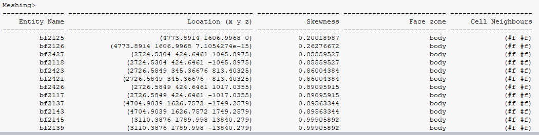
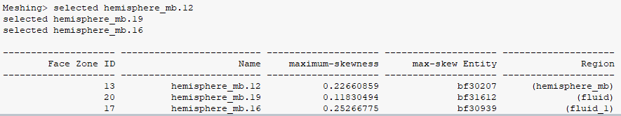
Use the List button to print details about the problematic cells to the console. for example:
Note: Useful keyboard shortcuts are provided in the graphics window, however, some particularly useful ones are: the up/down arrow keys to increase/decrease the display bounds, and Ctrl-g combination to draw face zones connected to selected zones.
Use the Graphics Selection fields to examine details for items that you select in the graphics window. By selecting an object (face, cell etc.) in the graphics window (or pasting an ID using output from the console window), click the Center in Window button to bring your graphics selection(s) more into focus. You can also print out a summary of the statistics for the selected object(s) by clicking the Print Details button. For example:
Use the Histogram button to generate a histogram of data for the selected issue in the chosen range, if applicable. Use the Draw button to draw all zones using the selected scope and the marked faces and cell in the chosen range, if applicable. Use the available shortcut keys (Appendix C: Shortcut Keys) to better interact with the display (for example, Ctrl+/ inserts a clipped plane at the centroid of a selected entity/zone.)
The Diagnostics Scope dialog box lets you determine the breadth of the mesh investigation. From here, you can define the scope of your diagnostic analysis to one or more selected mesh objects, face zones, or cell zones.
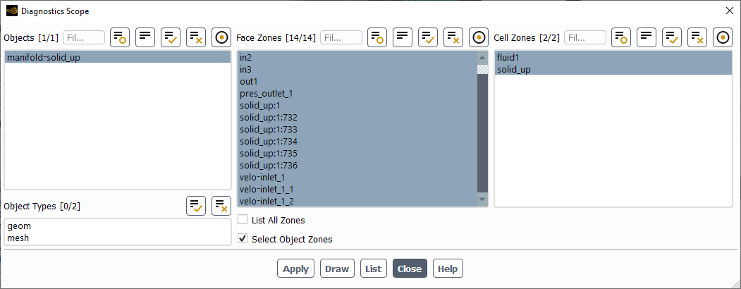
Use the Objects list to choose from available objects. Use the Object Types list to choose from geometry objects or mesh objects. Filtering and the support of wildcards, such as *, ?, [], Boolean NOT (^), Boolean AND (&), as well as Boolean OR (|), is available for the Objects list.
Use the Face Zones list to choose from available face zones. Use the List All Zones check box to show or hide all available zones. Use the Select Object Zones in order to quickly pick all zones associated with the selected object. Filtering and the support of wildcards, such as *, ?, [], Boolean NOT (^), Boolean AND (&), as well as Boolean OR (|), is available for the Face Zones list.
Use the Cell Zones list to choose from available cell zones. Filtering and the support of wildcards, such as *, ?, [], Boolean NOT (^), Boolean AND (&), as well as Boolean OR (|), is available for the Cell Zones list.
Use the Draw button to visualize your selections in the graphics window.
Use the List button to generate a detailed listing of your zone information. For example:
------------------------------
Number of Objects Selected : 1
------------------------------
Object Name : fluid-region-1
Number of Edge Zones  : 0
Number of Face Zones  : 7
Number of Cell Zones  : 0

Regions Info:

	Region Name : fluid-region-1
	Region Type : fluid
	Number of Face Zones  : 7

Total Number of Regions    : 1
Number of Fluid Regions    : 1, (fluid-region-1)
Number of Unfilled Regions : 1, (fluid-region-1)
------------------------------
Face Zones Summary :

      id                            name                 type    count      tri     quad     poly
  ______   _____________________________   __________________   ______   ______   ______   ______
  169034                      lotuscar.1                 wall   126636   126636        0        0
  169325                     tunnel-xmax                 wall      134      134        0        0
  169322                     tunnel-xmin                 wall      130      130        0        0
  169323                     tunnel-ymax                 wall      549      549        0        0
  169321                     tunnel-ymin                 wall      586      586        0        0
  169326                     tunnel-zmax                 wall      970      970        0        0
  169324                     tunnel-zmin                 wall    13552    13552        0        0
The Report Mesh Size dialog box reports the number of nodes, faces, and cells. Nodes and faces are grouped into those defining the boundaries and those used inside cell zones. Click to view the latest mesh statistics.
If the generation of the initial mesh fails, you can determine the number of meshed boundary nodes and faces by enabling Report Number Meshed in the Report Mesh Size dialog box. The headings Boundary and Interior will be replaced by Total and Meshed, respectively, and the total number of boundary nodes and faces will be reported along with the number that were meshed.
Note: Additional mesh statistics diagnostics and reporting tools are available in the ribbon. See Performing Meshing Diagnostics for details.
A good quality mesh guarantees the best analysis results for the problem, minimizes the need for additional analysis runs, and improves your predictive capabilities. The mesh should be fine enough to resolve the primary features of the problem being analyzed. The mesh resolution depends on the boundary mesh from which you start and the parameters controlling the generation of the interior mesh. In a high-quality mesh, the change in size from one face or cell to the next should be minimized. Large differences in size between adjacent faces or cells will result in a poor computational mesh because the differential equations being solved assume that the cells shrink or grow smoothly.
Note: Additional mesh quality diagnostic and reporting tools are available in the ribbon. See Performing Meshing Diagnostics for details.
Before generating a volume mesh, check the quality of the faces to get an indication of the overall mesh quality. To check face size and quality limits, use the Report > Face Limits... dialog box. For 3D meshes, a maximum of less than 0.9 and an average of 0.4 are good. The lower the maximum skewness, the better the mesh. See Quality Measure for information on face and cell quality measures available.
The default quality measure is skewness, but you can also report other quality measures such as the aspect ratio limits or the range in size change for a face zone. Before creating a layer of pyramid cells, check the aspect ratio of the quadrilateral faces that will form the base of the pyramids. This aspect ratio should be less than 8, otherwise the triangular faces of the pyramids will be highly skewed. If the aspect ratio is greater than 8, regenerate the quadrilateral faces:
If the quadrilateral faces were created in a different preprocessor, return to that application and try to reduce the aspect ratio of the faces in question.
If the quadrilateral faces were created during the building of prism layers, rebuild the prisms using a more gradual growth rate.
Check the skewness of triangular faces on a boundary from which you are going to build prisms to ensure that the quality of the prism cells will be good. After you create the prisms, check the skewness of the triangular faces that were created during the prism generation.
Face Distribution histogram
When checking the quality of the mesh you may find it useful to look at a histogram of boundary face quality or size. You can generate such a plot or report using the Face Distribution dialog box.
> >
The number of faces on the selected zones with a size or quality measure value (for example, skewness) in the specified range in each of the regularly spaced partitions is displayed in a histogram format. The x axis shows the size or quality and the y axis gives the number of faces or the percentage of the total number of faces.
You can modify the appearance of the histogram using the options available in the Axes dialog box. The following parameters can be modified:
Labels for the axes.
Scaling of the axes: decimal (default) or logarithmic.
Range of values: enable Auto Range or specify minimum and maximum values.
Major and minor rules: horizontal or vertical lines marking the primary and secondary data divisions, respectively. You can select the line color and thickness to be used.
Number format.
You can also modify the appearance of the histogram using the options available in the Curves dialog box. The following parameters can be modified:
Line style patterns, colors, and weight.
Marker symbols, colors, and styles.
When the histogram plot is displayed in the graphics window, you can use any of the mouse buttons to add text annotations to the plot. See Controlling the Mouse Buttons and Annotating the Display for more information about using the mouse buttons and annotation features.
After generating the volume mesh, check the quality of the cells to get an indication of overall mesh quality. The quality of the mesh plays a significant role in the accuracy and stability of the numerical computation. To check cell size and quality limits, use the Report > Cell Limits... dialog box.
The default quality measure is skewness, but you can also report other quality measures such as the aspect ratio limits or the range in size change for a cell zone. See Quality Measure for information on face and cell quality measures available.
Cell Distribution histogram
You can generate a histogram plot to graphically display cell size or quality by using the controls in the Cell Distribution dialog box.
> >
The number of cells in the selected zones with a size or quality value (for example, skewness) in the specified range in each of the regularly spaced partitions is displayed in a histogram format. The x axis shows either the size or the quality and the y axis gives the number of cells or the percentage of the total.
You can modify the appearance of the histogram using the options available in the Axes dialog box. The following parameters can be modified:
Labels for the axes.
Scaling of the axes: decimal (default) or logarithmic.
Range of values: enable Auto Range or specify minimum and maximum values.
Major and minor rules: horizontal or vertical lines marking the primary and secondary data divisions, respectively. You can select the line color and thickness to be used.
Number format.
You can also modify the appearance of the histogram using the options available in the Curves dialog box. The following parameters can be modified:
Line style patterns, colors, and weight.
Marker symbols, colors, and styles.
When the histogram plot is displayed in the graphics window, you can use any of the mouse buttons to add text annotations to the plot. For more information about the annotation features, see Controlling the Mouse Buttons and Annotating the Display.
For boundary layer flows, boundary cells with low skewness are very important. Use the Report Boundary Cell Limits dialog box to report the quality of cells containing a specified number of boundary faces or nodes.
For tetrahedral meshes, the maximum skewness will not be lower than the maximum face skewness, because the boundary cell skewness is limited by the boundary face skewness.
You can remove highly skewed cells with two boundary faces by using the Tet Improve dialog box.
> >
To specify the quality measure (skewness, aspect ratio, change in size, and so on), use the Quality Measure dialog box. The default quality measure is skewness.
>
Mesh quality is determined by the following quality measures:
- Orthogonal Quality
The orthogonal quality can simply be defined as:
Orthogonal Quality = 1 - Inverse Orthogonal Quality
Orthogonal Quality can be reported using the Quality option in the ribbon or the button in the General task page in solution mode (refer to Mesh Quality for details).
Note: Use the
report/enhanced-orthogonal-quality?text command to use an enhanced definition of the orthogonal quality measure that combines a variety of quality measures, including: the orthogonality of a face relative to vectors from the cell centroid to the face centroid and to the neighboring cell centroid; a metric that detects poor cell shape at a local edge (such as twisting and/or concavity); and the variation of normals between the faces that can be constructed from the cell face. This definition is optimal for evaluating thin prism cells.In addition, make sure you have enabled the enhanced orthogonal quality metric when generating and writing your file data.
- Enhanced Othogonal Quality
Employs an enhanced definition of the orthogonal quality measure that combines a variety of quality measures, including: the orthogonality of a face relative to a vector between the face and cell centroids; a metric that detects poor cell shape at a local edge (such as twisting and/or concavity); and the variation of normals between the faces that can be constructed from the cell face. This definition is optimal for evaluating thin prism cells.
The range is from -1 to 1. Under ideal conditions, the orthogonal quality is close to 1, whereas valid cells require the quality to be more than 0. The following table lists the range of orthogonal quality values and the corresponding cell quality.
Table 6.2: Orthogonal Quality Ranges and Cell Quality
Orthogonal Quality
Cell Quality
1
orthogonal
0.9–<1
excellent
0.75–0.9
good
0.5–0.75
fair
0.25–0.5
poor
>0–0.25
bad (sliver)
0
degenerate
- Skewness
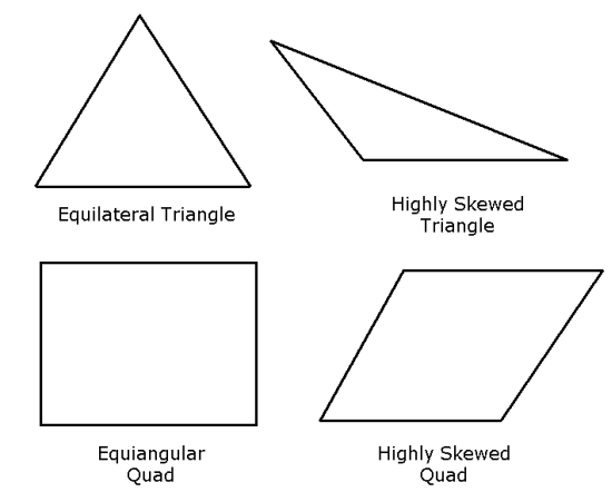
Skewness is one of the primary quality measures for a mesh. Skewness determines how close to ideal (that is, equilateral or equiangular) a face or cell is:
The following table lists the range of skewness values and the corresponding cell quality.
Table 6.3: Skewness Ranges and Cell Quality
Skewness
Cell Quality
1
degenerate
0.9–<1
bad (sliver)
0.75–0.9
poor
0.5–0.75
fair
0.25–0.5
good
>0–0.25
excellent
0
equilateral
According to the definition of skewness, a value of 0 indicates an equilateral cell (best quality) and a value of 1 indicates a completely degenerate cell. Degenerate cells (slivers) are characterized by nodes that are nearly coplanar. Cells with a skewness value above 1 are invalid.
Highly skewed faces and cells should be avoided because they can lead to less accurate results than when relatively equilateral/equiangular faces and cells are used.
Two methods for measuring skewness are:
Based on the equilateral volume (applies only to tetrahedra).
Based on the deviation from a normalized equilateral angle. This method applies to all cell and face shapes, such as pyramids and prisms.
The default skewness method for tetrahedra is the equilateral volume method, but you can change to the angle deviation method using the Quality Measure dialog box.
Equilateral-Volume-Based Skewness
In the equilateral volume deviation method, skewness is defined as

(6–1)
where, the optimal cell size is the size of an equilateral cell with the same circumradius.
In 3D meshes, most cells should be rated good or better, but a small percentage will generally be in the fair range and there are usually even a few poor cells. The presence of poor cells can indicate poor boundary node placement. You should try to improve your boundary mesh as much as possible because the quality of the overall mesh can be no better than that of the boundary mesh.
Normalized Equiangular Skewness
In the normalized angle deviation method, skewness is defined (in general) as

(6–2)
where
 = largest angle in the face or cell
  = smallest angle in the face or cell
 = angle for an equiangular face/cell (such as 60 for a triangle,
90 for a quad, and so on)
= angle for an equiangular face/cell (such as 60 for a triangle,
90 for a quad, and so on) The cell skewness will be the maximum skewness computed for any face. For example, an ideal pyramid (skewness = 0) is one in which the 4 triangular faces are equilateral (and equiangular) and the quadrilateral base face is a square. The guidelines in Table 6.3: Skewness Ranges and Cell Quality apply to the normalized equiangular skewness as well.
- Size Change
Size change is the ratio of the area (or volume) of a face (or cell) in the geometry to the area (or volume) of each neighboring face (or cell). This ratio is calculated for every face (or cell) in the domain. The minimum and maximum values are reported for the selected zones.
- Edge Ratio
The edge ratio is defined as the ratio of maximum length of the edge of the element to the minimum length of the edge of the element.
By definition, edge ratio is always greater than or equal to 1. The higher the value of the edge ratio, the less regularly shaped is its associated element. For equilateral element shapes, the edge ratio is always equal to 1.
- Aspect Ratio
The aspect ratio of a face or cell is the ratio of the longest edge length to the shortest edge length. The aspect ratio applies to triangular, tetrahedral, quadrilateral, and hexahedral elements and is defined differently for each element type.
The aspect ratio can also be used to determine how close to ideal a face or cell is.
For an equilateral face or cell (such as an equilateral triangle, a square, and so on), the aspect ratio is 1.
For less regularly-shaped faces or cells, the aspect ratio will be greater than 1 as the edges differ in length.
For triangular faces and tetrahedral cells and for pyramids, you can usually focus on improving the skewness, and the smoothness and aspect ratio will consequently be improved as well.
For prisms, it is important to check the aspect ratio and/or the change in size in addition to the skewness, because it is possible to have a large jump in cell size between two cells with low skewness or a high-aspect-ratio low-skew cell.
- Squish
Squish is a measure used to quantify the non-orthogonality of a cell with respect to its faces. It is defined as follows:

(6–3)
where
A = face unit area vector
 = the vector connecting the adjacent cell centroids (for face
squish) or the cell and face centroids (for cell squish)
= the vector connecting the adjacent cell centroids (for face
squish) or the cell and face centroids (for cell squish)- Warp (Quadrilateral Elements only)
Face warp applies only to quadrilateral elements and is defined as the variation of normals between the two triangular faces that can be constructed from the quadrilateral face. The actual value is the maximum of the two possible ways triangles can be created.
Mathematically, it is expressed as follows:

(6–4)
where
 = the deviation from a best-fit plane that contains the element
  ,
,  = the lengths of the line segments that bisect the edges of the
element
= the lengths of the line segments that bisect the edges of the
element The value of face warp ranges between 0 and 1. A value of 0 specifies an equilateral element and a value of 1 specifies a highly skewed element.
- Dihedral Angle
Dihedral angle applies only to faces and not cells. The dihedral angle is defined as the angle between the normals of adjacent faces. This quality measure is useful in locating sharp corners in complicated geometries. The dihedral angle value ranges from 0–180.
- ICEM CFD Quality
The ICEM CFD quality measure calculates element quality based on the quality values in ANSYS ICEM CFD. This measure is only available for cells, not faces.
Tetrahedra: The quality is calculated as the skewness of the tetrahedral element.
The remaining quality values are based on various quality metrics computed in ANSYS ICEM CFD.
Hexahedra: The quality is based on the Determinant, Max Orthogls, and Max Warpgls metrics in ANSYS ICEM CFD.
The determinant is the ratio of the smallest and the largest determinant of the Jacobian matrices, where a Jacobian matrix is computed at each node of the element.
The max orthogls metric calculates the maximum deviation of the internal angles of the element from 90 degrees. Angles between 180 and 360 degrees (deviation up to 270 degrees) will also be considered.
The warp for each face is calculated as the maximum angle between the triangles connected at the diagonals of the face. The max warpgls metric is calculated as the maximum warp of the faces comprising the element.
These values are normalized and the minimum value of the three normalized diagnostics will be used.
Pyramids: The quality is based on the Determinant computed in ANSYS ICEM CFD.
The determinant is the ratio of the smallest and the largest determinant of the Jacobian matrices, where a Jacobian matrix is computed at each node of the element.
Prisms: The quality is based on the Determinant and Warp computed in ANSYS ICEM CFD.
The determinant is the ratio of the smallest and the largest determinant of the Jacobian matrices, where a Jacobian matrix is computed at each node of the element.
The warp for each face is calculated as the maximum angle between the respective edges and a plane containing the mid-points of the edges comprising the face. The warp for the element is then calculated as the maximum warp of the faces comprising the element.
The quality is calculated as the minimum of the determinant and warp.
For further details on the quality measures available in ANSYS ICEM CFD, refer to the ANSYS ICEM CFD Help Manual.
The range of quality values reported is between 0-2 (the range in ANSYS ICEM CFD is -1 to 1, and a value of 2 corresponds to -1 in ANSYS ICEM CFD, 1 to 0, and 0 to 1, respectively). A value of 0 indicates a perfect, non-distorted element, 1 indicates a degenerate element, and values above 1 indicate an invalid element (such as concave, dihedral angle > 180 degree, or negative volume elements).
- Ortho Skew
The ortho skew quality for a cell is computed using the face normal vector,
 for each face; the vector from the cell centroid to the centroid
of each of the adjacent cells,
for each face; the vector from the cell centroid to the centroid
of each of the adjacent cells,  ; and the vector from the cell centroid to the centroid of each
face,
; and the vector from the cell centroid to the centroid of each
face,  . Figure 6.20: Vectors Used to Compute Ortho Skew/Inverse Orthogonal Quality for a
Cell illustrates the vectors used to determine the ortho skew
quality for a cell.
. Figure 6.20: Vectors Used to Compute Ortho Skew/Inverse Orthogonal Quality for a
Cell illustrates the vectors used to determine the ortho skew
quality for a cell.For each face
 , the calculation first finds the value of (1 - the cosine of the
angle between the face normal vector and the corresponding vector from the centroid
of the cell to the centroid of that face):
, the calculation first finds the value of (1 - the cosine of the
angle between the face normal vector and the corresponding vector from the centroid
of the cell to the centroid of that face): 
(6–5)
Next, for each face
, the calculation finds the value of (1 - the cosine of the angle
between the face normal vector and the corresponding vector from the centroid of the
cell to the centroid of the adjacent cell that shares that face): 
(6–6)
The reported Ortho Skew quality for a cell then depends on the cell type:
For most cells, Ortho Skew is the maximum of the above quantities computed for each face.
For pyramid cells, Ortho Skew is the maximum of the cell skewness and the above quantities computed for each face.
Note:When the cell is located on the boundary, the vector
across the boundary face is ignored during the quality
computation. When the cell is separated from the adjacent cell by an internal wall, the vector
 across the internal boundary face is ignored during the
quality computation.
across the internal boundary face is ignored during the
quality computation. When the adjacent cells share a parent-child relation, the vector
is the vector from the cell centroid to the centroid of the
child face while the vector  is the vector from the cell centroid to the centroid of the
adjacent child cell sharing the child face.
is the vector from the cell centroid to the centroid of the
adjacent child cell sharing the child face.
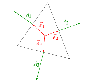
The ortho skew quality for faces is similarly computed using the edge normal vector,
 , and the vector from the face centroid to the centroid of each
edge,
, and the vector from the face centroid to the centroid of each
edge,  . Figure 6.21: Vectors Used to Compute Ortho Skew Quality for a Face illustrates the vectors used to determine the ortho skew
quality for a face.
. Figure 6.21: Vectors Used to Compute Ortho Skew Quality for a Face illustrates the vectors used to determine the ortho skew
quality for a face.The ortho skew for a face is the maximum of the computed values for (1 - the cosine of the angle between the edge normal vector and the vector from the centroid of the face to the centroid of the edge), for each edge
 :
: 
(6–7)
When the Rapid Octree mesher is used, the quality measure is changed to ortho skew by default.
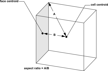
- Fluent Aspect Ratio
The Fluent aspect ratio is a measure of the stretching of a cell. It is computed as the ratio of the maximum value to the minimum value of any of the following distances: the normal distances between the cell centroid and face centroids, and the distances between the cell centroid and nodes. For a unit cube (see Figure 6.22: Calculating the Fluent Aspect Ratio for a Unit Cube), the maximum distance is 0.866, and the minimum distance is 0.5, so the aspect ratio is 1.732. This type of definition can be applied on any type of mesh, including polyhedral.
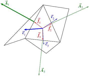
- Inverse Orthogonal Quality
The inverse orthogonal quality for a cell is computed using the face normal vector,
for each face; the vector from the cell centroid to the centroid
of each of the adjacent cells, ; and the vector from the cell centroid to the centroid of each
face, (see Figure 6.20: Vectors Used to Compute Ortho Skew/Inverse Orthogonal Quality for a
Cell). For each face, the cosines of the angle between and , and between and are calculated. The smallest calculated cosine value is the
orthogonality of the cell. Then, inverse orthogonality is found by subtracting this
cosine value from 1.Finally, Inverse Orthogonal Quality depends on cell type:
For tetrahedral, prism, and pyramid cells, Inverse Orthogonal Quality is the maximum of the cell skewness and the inverse orthogonality.
For hexahedral and polyhedral cells, Inverse Orthogonal Quality is the same as the inverse orthogonality.
The worst cells will have an Inverse Orthogonal Quality closer to 1 and the best cells will have an Inverse Orthogonal Quality closer to 0.
Note:
Inverse Orthogonal Quality = 1 - Orthogonal Quality
Orthogonal Quality can be reported using the Quality option in the ribbon or the button in the General task page in solution mode (refer to Mesh Quality for details).
In addition to the mesh diagnostic and reporting tools available in the ribbon (see Performing Meshing Diagnostics for details), the mouse probe print function displays information about individual components of the mesh. The type of information is determined by the selected mouse probe filter.
The print-info command reports information about an individual
mesh entity (that is, a node, face, or cell). In some circumstances, the information
includes prefixes or punctuation to identify the information type. An entity is identified
by its prefix with an index value. Valid prefixes are: bn (boundary
node), n (node), bf (boundary face),
f (face), and c (cell). Hence, the first
boundary node would be bn1.
The output for some of the entity types is as explained in this section.
cell
The following information is listed for a cell:
zone ID
the nodes forming the cell
the faces forming the cell
the size
the coordinates of the circumcenter (relevant for tetrahedral cells only)
square of the circumcenter radius (relevant for tetrahedral cells only)
the quality of the cell
 c26 = (1 (n262 n34 bn204 bn205) (f4743 f5372 f1822 f3426)
 0.00020961983 (2.7032523 0.32941867 0.072823988)
 0.0081779587 0.44769606)
The default measure of quality is skewness, but you can use the Quality Measure dialog box to specify aspect ratio or change in size instead.
face
The following information is listed for a face:
associated zone ID
the nodes forming the face
the neighboring cells
f32 = (4 (n95 bn197 n90) (c4599 c1279))
Due to the manner in which the algorithm maintains memory, not all indices will have values—that is, an empty slot can be caused by a delete operation. Empty slots are reused in subsequent operations, so the actual entity at a particular index may change as the mesh is generated.
boundary face
The following information is listed for a boundary face:
associated zone ID
the nodes forming the face
the neighboring cells
the periodic shadow (null if not periodic)
the quality of the face
bf17 = (2 (bn1308 bn1314 bn1272) (() c1533) () 0.014393554)
The default measure of quality is skewness, but you can use the Quality Measure dialog box to specify aspect ratio or change in size instead.
node
The following information is listed for a node:
associated zone ID
Cartesian coordinates of the node
the node radius
n30 = (5 (2.433799 0.078610075 0.52846689) 0.12702106)
For interior nodes, the node radius is the distance-weighted average to the surrounding nodes.
boundary node
The following information is listed for the boundary node:
associated zone ID
Cartesian coordinates of the node
node radius
faces using the node.
bn1 = (3 (0 0 0) 0.1 (bf2099 bf1093 bf193))
For boundary nodes, the node radius is the average distance to neighboring boundary nodes.