


Ansys Fluent can interpolate solution data for a given geometry from one mesh to another, allowing you to compute a solution using one mesh (for example, hexahedral) and then change to another mesh (for example, hybrid) and continue the calculation using the first solution as a starting point.
Important: Ansys Fluent does zeroth-order interpolation for interpolating the solution data from one mesh to another.
For additional information, see the following sections:
The procedure for mesh-to-mesh solution interpolation is as follows:
Set up the model and calculate a solution on the initial mesh.
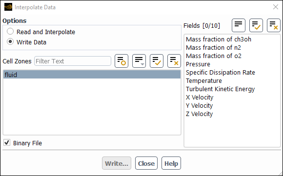
Write an interpolation file for the solution data to be interpolated onto the new mesh, using the Interpolate Data dialog box (Figure 3.17: The Interpolate Data Dialog Box).
 File → Interpolate...
Under Options, select Write Data.
In the Cell Zones selection list, select the cell zones for which you want to save data to be interpolated.
Note: If your case includes both fluid and solid zones, write the data for the fluid zones and the data for the solid zones to separate files.
Select the variable(s) for which you want to interpolate data in the Fields selection list. All Ansys Fluent solution variables are available for interpolation.
Select the Binary File check box if you want a binary interpolation file to be generated.
Note: Writing a binary interpolation file is significantly faster and requires less memory than writing a text file.
Click Write... and specify the interpolation file name in the resulting Select File dialog box. The file format is described in Format of the Interpolation File.
Set up a new case.
Read in the new mesh, using the appropriate ribbon tab item (File/Read/ or File/Import/).
Define the appropriate models.
Important: Enable all of the models that were enabled in the original case. For example, if the energy equation was enabled in the original case and you forget to enable it in the new case, the temperature data in the interpolation file will not be interpolated.
Define the boundary conditions, material properties, and so on.
Important: An alternative way to set up the new case is to save the boundary conditions from the original model using the
write-settingstext command, and then read in those boundary conditions with the new mesh using theread-settingstext command. See Reading and Writing Boundary Conditions for further details.Read in the data to be interpolated.
File → Interpolate...
Under Options, select Read and Interpolate.
In the Cell Zones list, select the cell zones for which you want to read and interpolate data.
If the solution has not been initialized, computed, or read, all zones in the Cell Zones list are selected by default, to ensure that no zone remains without data after the interpolation. If all zones already have data (from initialization or a previously computed or read solution), select a subset of the Cell Zones to read and interpolate data onto a specific zone (or zones).
Click the button and specify the interpolation file name in the resulting Select File dialog box.
Important: If your case includes both fluid and solid zones, the two sets of data are saved to separate files. Hence perform these steps twice, once to interpolate the data for the fluid zones and once to interpolate the data for the solid zones.
Reduce the under-relaxation factors and calculate on the new mesh for a few iterations to avoid sudden changes due to any imbalance of fluxes after interpolation. Then increase the under-relaxation factors and compute a solution on the new mesh.
An example of an interpolation file is shown below:
 3
 2
 34800
 3
 x-velocity
 pressure
 y-velocity
 (-0.068062
 -0.0680413
 ...
The format of the interpolation file is as follows:
The first line is the interpolation file version. It is
2for files generated using Ansys Fluent 12.0 through 14.0,3for text files generated using Ansys Fluent 14.5,4for binary files generated using single precision Ansys Fluent 14.5, and5for files generated using double precision Ansys Fluent 14.5.The second line is the dimension (
2or3).The third line is the total number of points.
The fourth line is the total number of fields (temperature, pressure, and so on) included.
Starting at the fifth line is a list of field names. To see a complete list of the field names used by Ansys Fluent, enter the
display/contourtext command and view the available choices by pressing Enter at thecontours of>prompt. The list depends on the models turned on.After the field names is a section for each list of
 ,
,  , and (in 3D)
  coordinates for all the
data points.
coordinates for all the
data points.At the end is a section for each list of the field values at all the points in the same order as their names. The number of coordinate and field points should match the number given in line 3.
For version
3interpolation files, the sections are bounded by “(” and “)”.For version
4and5interpolation files, the sections are bounded by “(” and “\nEnd of Binary Section 0)”.The delimiters help skip a section if the associated model is not enabled. With version
2interpolation files (where the delimiters do not exist), sections may not be skipped properly if the size of the field cannot be determined without enabling the associated model. This may result in incorrect interpolation of the subsequent field variables.Important: An interpolation file written with Ansys Fluent 14.5 and above is not readable in prior versions of Ansys Fluent.