The following sections of this chapter are:
The following tutorials illustrate some of the advanced capabilities of FENSAP-ICE, such as the Extended Icing Data and the 2D capabilities of ICE3D.
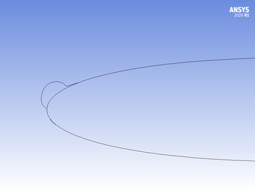
Icing calculations at high air speeds require special treatment when the total temperature of the flow is very close or above freezing temperature. This condition may arise when the icing temperature is low but the Mach number is in the mid- to transonic range. The ice shapes encountered in this flow regime, typically referred to as beak ice, are usually characterized by well-defined small horns growing at a short distance from the stagnation point on a mostly uncontaminated surface. This is a type of ice shape that is usually observed on the outboard sections of helicopter main rotor blades. For these severe cases, an additional feature called Extended Icing Data (EID) should be activated, where FENSAP performs additional post-processing of the flow to improve the icing thermodynamics in ICE3D for this regime.
Download the 5_ICE3D_Advanced.zip file
here
.
Unzip 5_ICE3D_Advanced.zip to your working directory.
Create a new project, and call it
High_Speed_Icing.Create a new run by selecting FENSAP as the flow solver.
Assign the grid file naca0012_fine provided by Ansys in the tutorials subdirectory ../workshop_input_files/Input_Grid/Extended_Icing_Data by double-clicking the grid icon and navigating to this directory. This grid is a fine version of the one used in the introductory tutorials.
Double-click the config icon to open the FENSAP graphical and input parameter windows.
Go to the Model section. Select the Navier-Stokes option in the Momentum equations box (viscous flow) and the Full PDE in the Energy equation box. Select the Spalart-Allmaras option in the Turbulence model box. Set the value of the Eddy/Laminar viscosity ratio to
1e-5. Turbulence is then only generated by the airfoil.In the Surface roughness tab, set the Specified sand-grain roughness value to
0.0005m.Go to the Conditions panel. Set the reference flow conditions to:
Characteristic length 0.1524mAir velocity 190m/sAir static pressure 80800PaAir static temperature 257K (-16.15°C)Set the Initial solution with the Velocity angles option and set the angle of attack to
7degrees.Go to the Boundaries panel to set the boundary conditions.
Set BC_1000 to type Supersonic or far field, for which all primitive variables are required, and click Import reference conditions to automatically copy the boundary conditions from the reference values set at step 6.
Click BC_2001. Impose a no-slip condition and set a surface heat flux of
0W/m2. For the EID calculations, icing walls need to be set as adiabatic walls. HTC will be extracted later on as part of EID solution.Click the Yes button.
Repeat for the remaining three wall boundaries 2002, 2003, and 2004.
Go to the Solver menu. Select Steady in the Time integration box. Set the CFL number to 100. Set the Maximum number of time steps to 1,000. Activate Use variable relaxation and specify 300 Time steps.
Select the Streamline upwind (SU) artificial viscosity scheme with second-order crosswind coefficient set to
1.0e-7. These settings should appear by default.Go to the Out panel, set Solution every
20iterations.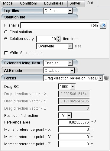
Click the Forces tab and select the Drag direction based on inlet BC option. Set the Reference area to
0.02322576m2.Click the button at the bottom of the window to open the execution menu and start the computations.
Create a new DROP3D run in the project directory of the previous section.
Drag & drop the config icon of the FENSAP run onto the config icon of the DROP3D run. This will automatically transfer the necessary airflow settings.
Open the DROP3D config icon. In the Model panel, set the Physical model to Droplets. Set Particle type in the Particles parameters section to Droplets.
Go to the Conditions panel and set a value of
0.2g/m3 for LWC and a droplet diameter of20microns.Water density should appear by default with a value of 1000 kg/m3.
In the Boundaries panel, select the Inlet boundary and click the Import reference conditions button to automatically copy the inlet boundary conditions of DROP3D.
Go to the Solver panel. Set the CFL number to
20and the Maximum number of time steps to150.Go to the Out panel and select Solution every
40iterations.Click and start the computations. The final results, visualized with Viewmerical, should be similar to those appearing in the following figure.
Create a new ICE3D run in the same project directory used for the previous FENSAP and DROP3D calculations.
Drag & drop the config icon of the DROP3D calculation onto the config icon of ICE3D.This automatically copies the input parameters of DROP3D into ICE3D.
Double-click the config icon to access the settings.
In the Model panel, select the Glaze – Advanced option in the Icing model section. Set the Heat flux type to Classical.
While in the Model panel, activate the EID calculation by setting Compute EID to :

This option computes the heat transfer coefficients from the adiabatic solution before executing the icing simulation.
In the Conditions panel, verify that the reference flow and droplet conditions have been correctly copied from the airflow and droplet configuration files. Set the Recovery factor value to
0.9.In the Model parameters section, verify that the Icing air temperature is set to
257K (-16.15°C). Leave the parameters in this section to their default values. Ice density should be set to Constant type and its default value of917kg/m3.In the Boundaries panel, click BC_2004. In the Icing box, change the option to Sink. Sink boundaries remove any impingement and runback and prevent ice formation on them. In this case, you will use it to remove runback water from reaching the trailing edge on the lower side and requiring a very small time step for a stable solution.
Go to the Solver panel and set the Total time of ice accretion to 60 seconds. Keep the Automatic time step enabled.
Run this calculation on
4processors, if possible.The ice shape should be like the one shown in the following figure:
This tutorial illustrates the procedure required to compute ice accretion on a rotating axisymmetric surface with FENSAP-ICE, using steady-state airflow and droplet solutions. When the rotating geometry is axisymmetric, a steady-state flow solution can be obtained by imposing an angular velocity boundary condition on the no-slip wall. The resulting ice shape will also be axisymmetric, regardless of the angle of attack of the rotating surface. This computational method can be used to compute ice accretion on propeller and engine spinners. The surface grid does not need to be axisymmetric, which is the case in general for unstructured grids. There is no limitation on the number of spinners, their locations and orientations, allowing solutions for full aircraft configurations with spinners and engine nacelles.
To obtain a flow solution for a general 3D geometry with rotating spinner(s):
Create a new project and name it
Spinner.Create a new FENSAP run by clicking on the new run icon.
Assign the grid file spinner provided in the tutorials subdirectory ../workshop_input_files/Input_Grid/Spinner, by double-clicking on the grid icon and by navigating to this directory.
Double-click the config icon to open the FENSAP graphical and input parameter window.
In the Model panel, go to the Turbulence model section and select the Spalart-Allmaras model. In the Surface roughness section, select the Specified sand-grain roughness option and set a value of
0.0005m.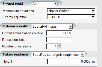
Go to the Conditions panel. In the Reference conditions section, change the following values:
Characteristic length 0.1mAir static temperature -11°C (262.15K)In the Initial Solution section, switch to Velocity angles and set:
Angle of attack 5deg.Yaw angle 0deg.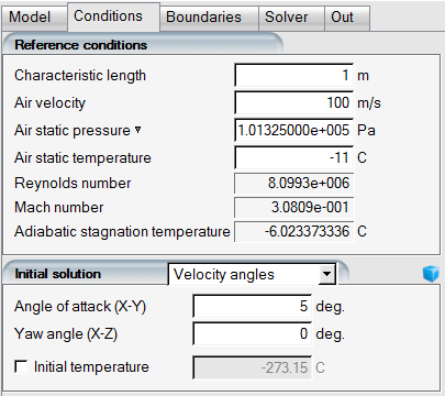
Tip: The units displayed can be changed through the Settings menu in the main FENSAP-ICE window.
Go to the Boundaries panel. For the inlet boundary BC_1000 choose inlet type Supersonic or far-field, and click to assign the boundary conditions.
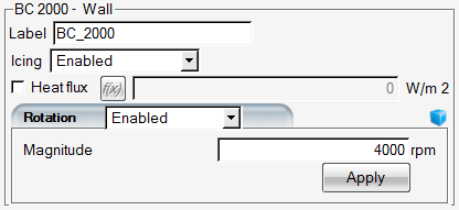
Click BC_2000 to set the wall boundary conditions for the spinner. This wall surface is at the front of the geometry and an angular velocity is assigned to it. Set the Temperature value to
14.85°C in order to compute the heat fluxes needed in the glaze ice simulation. Note that in order to obtain meaningful heat fluxes the wall temperature must always be a few degrees greater than the adiabatic stagnation temperature.Note: In the case of an axisymmetric rotating surface the maximum value of the tangential velocity must also be taken into account to determine the maximum wall stagnation temperature value.
The axis of rotation is automatically detected by FENSAP-ICE, and displayed in the viewer port on the left. In the Rotation box, select the Enabled option and assign a rotation rate of
4000rpm. The direction of the rotation always follows the right-hand rule. Click the Apply button. Zoom in on the selected wall to see the rotation axis and the direction of the rotation.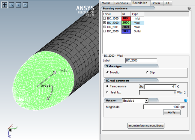
Note: To reverse the direction of rotation, simply add a minus (-) sign in front of the rotation magnitude.
Click BC_2001 to set the wall conditions. This surface is the cylindrical part of the geometry which is not rotating. Set the wall temperature to
14.85°C and keep Rotation disabled on this wall.Go to the Solver tab. Set the CFL number to
100. Set the number of time steps to300. Uncheck the Use variable relaxation option. Change the Crosswind dissipation to1e-6, which is better for coarse meshes like this.Click the button at the bottom of the panel to go to the Execution environment. In the Settings panel, set the number of CPUs to
4if possible.Click the menu button to start the calculation. The progress of the calculation can be monitored in the Execution panel.
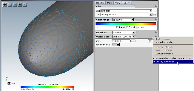
Load the converged solution on Viewmerical using the button. To display the surface velocity and shear stress vectors, first disable all boundaries but walls. Zoom in on the front of the spinner.
In the Data panel, choose Velocity Vectors in the data field box. You can change the vector display lengths by and buttons in the Scale box.
To overlay the wall boundary with the vectors, click the cube menu to the right of Vector Data box and check Overlay boundaries.
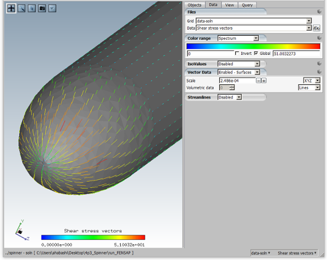
Similarly, you can display the shear stress vectors on the surface, showing the effect of rotation.
DROP3D does not require wall boundary conditions, therefore no boundary condition is needed for the rotating spinner surface. The effect of the rotation of the spinner induces rotation in the boundary layer, which affects the droplets when they are very close to the surface. Large droplets will not be affected by this much. In the current example the tangential velocity of the surface is small compared to the axial velocity and the effect on the droplets is miniscule.
Create a new DROP3D run by clicking on the new run icon.
Drag and drop the config icon of the previous FENSAP run onto the config icon of this DROP3D run to copy the reference and boundary conditions from the flow solution.
For this tutorial, the default values of free stream LWC (1 g/m3) and MVD (20 microns) are retained. Do not modify the reference and boundary conditions that have been automatically assigned by the drag & drop operation.
Go to the Boundaries panel. For the BC_1000, press the to copy the reference velocities and LWC into the boundary conditions.
Go to the Solver panel. Set the CFL number to
20and the number of time steps to100.Click the button at the bottom of the panel to go to the Execution settings. In the Settings panel, set the Number of CPUs to
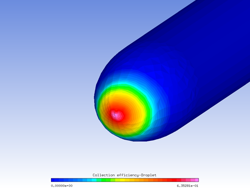
4if possible.Click the menu button to start the calculations. The progress of the calculations can be monitored in the Execution panel.
Note: The collection efficiency shown in the figure above will be circumferentially averaged by ICE3D to include the effect of rotation before the ice accretion calculation is performed.
Water runback and ice accretion on the spinner for glaze icing conditions are computed with ICE3D. The water film is very thin and rotates with the spinner surface. The rotation induces a centrifugal force on the water film, which translates into an additional force vector tangent to the surface. The film is now moving under the effect of both shear stresses and centrifugal forces.
Create a new ICE3D run by clicking on the new run icon.
Drag & drop the config icon of the previous DROP3D run onto the config icon of this ICE3D run to copy the reference and boundary conditions from the airflow and droplet solutions.
Go to the Models panel. In the Icing model section, select the Glaze - Advanced model and select the Classical heat flux option.
Go to the Boundaries panel. The drag & drop operation should have automatically assigned the rotation settings on the spinner wall designated by BC_2000.
Go to the Solver panel. Keep the Automatic time step enabled and set the Total time of ice accretion to
120seconds.Click the button at the bottom of the panel to go to the Execution environment. In the Settings panel, set the Number of CPUs to
4if possible.Click the menu button to start the calculation. The progress of the calculation can be monitored in the Execution panel.
Figure 5.4: Ice Shapes Obtained with Rotation (Left) and Without Rotation (Right) at an Angle of Attack of 5 °
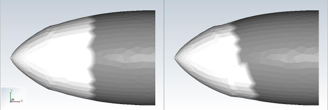
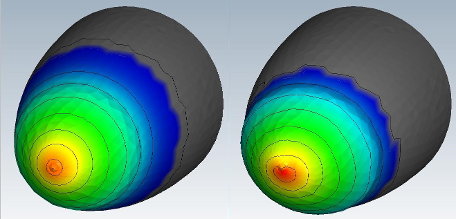
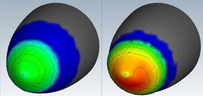
Figure 5.5: Distribution of the Collected Mass of Water with Rotation (Left) and Without Rotation (Right)
The following sections of this tutorial are:
The objectives of this tutorial are to solve the particle field (droplets and ice crystals) around a NACA0012 airfoil, and to investigate the impact of ice crystals on the collection efficiency.
If this step has not already been performed, create a new project using → or, the New project icon and select the metric unit system. Name the project
Ice_Crystals.Create a new run using → or the new run icon. This tutorial uses DROP3D as the impingement solver. You can name this run
DROP3D_MULTIPHASE.Assign a grid file by double-clicking the grid icon. Select the grid file provided in the tutorials subdirectory ../workshop_input_files/Input_Grid/Ice_Crystals. The grid file shown below is in FENSAP format and contains a NACA0012 airfoil with a chord length of 0.9144 m.
Figure 5.7: Grid and Airflow Solution: NACA0012 C-Grid with Chord Length of 0.9144m (Left), Mach Contours from the Airflow Solution (Right)
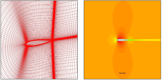
Assign an airflow solution file by double-clicking on the airsol icon. Select the file soln file provided in the tutorials subdirectory ../workshop_input_files/Input_Grid/Ice_Crystals.
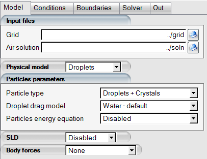
Double-click the config icon. A new window appears for the configuration of the input parameters for DROP3D.
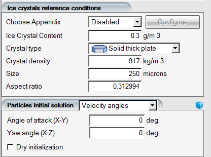
In Particle parameters section, select Droplets + Crystals as the Particle Type. The drag model for droplets is default, and the drag model for crystals is assigned automatically.
Select the Conditions panel and configure the following figures:
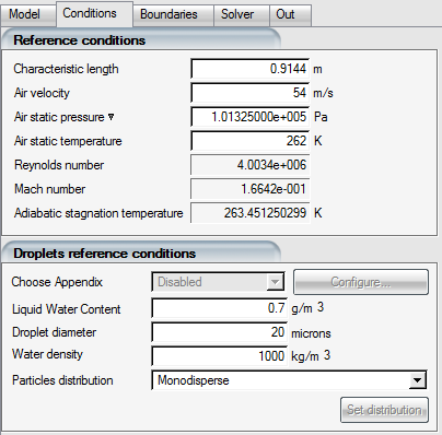
Select the Boundaries panel and select the inlet boundary BC_1000. Set the Type to Supersonic or far field. Click the icon at the bottom of the panel. This will import the initial conditions for droplets and ice crystals from those entered in the Conditions panel.
Select the Solver panel. Set the CFL number to
20and Maximum number of time steps to300.Select the Out panel. Save the droplet and crystal solution files, in FENSAP format, and choose to Overwrite files every
50iterations. Name the solution file for dropletsdropletand the solution file for crystals,crystal.Run this calculation on
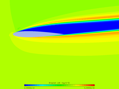
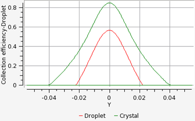
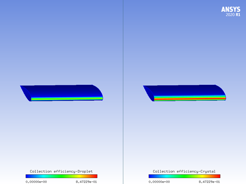
2or more processors, if possible. The run should stop due to convergence in about 130 iterations.Load the two solutions, droplet and crystal, using the button to compare the collection efficiency of droplets and crystals with the 2D plot.
Note: Ice crystals have a higher collection efficiency than droplets due to their high inertia.
The objective of this tutorial is to evaluate the impact of ice crystals to ice accretion. Note that this tutorial requires droplet and ice crystal solutions that should be obtained by following the tutorial DROP3D Particle Impingement with Ice Crystals and Water Droplets.
Create a new run using → or the new run icon. This tutorial uses ICE3D as the ice accretion solver. Name the run
ICE3D_MULTIPHASE.Drag & drop the config icon of the DROP3D_MULTIPHASE calculation (droplet and ice crystal input parameters) onto the config icon of ICE3D_MULTIPHASE. This automatically copies the required input parameters for both droplets and ice crystals.
Double-clicking on the config icon opens the input parameter window of ICE3D, the ice accretion solver.
Select the Model panel. In the Icing Model section, select Glaze - Advanced for Ice – Water model, and Classical for Heat flux type.
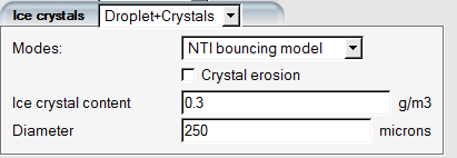
Choose Droplets+Crystals in the Ice crystals tab to activate ice crystals.
Choose the NTI bouncing model as the particle bouncing mode. This adds the effect of ice crystals surface collisions dynamics to the ice shape.
In the Forces and fluxes section, assign the surface.dat and hflux.dat files by choosing them in the tutorials subdirectory ../workshop_input_files/Input_Grid/Ice_Crystals.
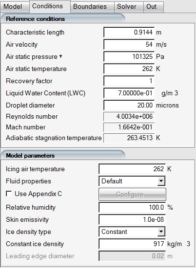
Select the Conditions panel. Ensure that the following Reference conditions and Model parameters are set:
Select the Solver panel. Solve the ice accretion for
600seconds in time, with Automatic time step enabled.Switch to the Out panel. Output the solution at the end of the ice accretion time (600 seconds). Generate a displaced grid by selecting Yes and choose the Grid Displacement Method as Default (Coupled) and Displacement sub-iterations of
5.Run this calculation on
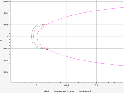
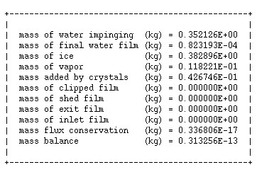
2processors, if possible.A comparison of the ice shapes obtained using 0.7 g/m3 droplets + 0.3 g/m3 ice crystals (in blue), and using 1.0 g/m3 droplets only (red) is shown below. The mass added by crystals is miniscule due to bouncing effects, which can be verified in the mass balance table in the log file of ICE3D (shown below). When this is the case, ice mostly forms by the 0.7 g/m3 droplet impingement. Compared to 1 g/m3 droplets, there is less runback, which is why the ice shape looks different on either side of the leading edge.
Figure 5.10: Comparison of Ice Shapes Obtained Using Droplets and Ice Crystals (Blue) and Droplets Only (Red)