If the thermal model is enabled in Rocky, an additional equation for thermal energy balance is solved along with the equations governing the motion of particles. In the current implementation of Rocky, the temperature is assumed to be uniform in standard single-element particles (non-flexible). This means that no radial nor circumferential temperature variation is admitted inside any of these particles, which is reasonable if they are small and/or made of highly conductive materials. On the other hand, for multi-element flexible particles, which are formed by connected elements as described in chapter Flexible particles in Rocky, the temperature may have variation between elements. However, the temperature of each element making up a flexible particle is considered to be uniform also.
In Rocky, the temperature variation of a particle or element over time is determined by solving the differential equation:
(2–54) |
in which, and
are, respectively, the mass and the specific heat of the particle or element
, while
is the overall heat transfer rate between it and its surroundings. For
instance, in all DEM problems,
accounts for the conduction heat transfer rate that occurs during the
contact with other particles or boundaries. Additionally, if the problem being solved includes
fluid flow, the heat transfer rate between the particle and the fluid phase,
, is included in
as well. Moreover, if
is an element of a flexible particle, the heat transfer rate across the
inter-element joints must be considered also. Then, for the most general case we can write:
(2–55) |
where is the instantaneous heat transfer rate from another particle or a wall
through a contact c, whereas
is the instantaneous heat transfer rate from the other element of the same
particle connected to
through a joint j. In this equation,
is the number of contacts that
has with other particles or walls at a given time, while
is the number of joints at which
connects itself with other elements.
Another option available when the thermal model is enabled in Rocky is the Thermal Integration Model, which ignores any conduction inside the particle and assumes only that all particles have a single temperature. The default option in Rocky updates the particle temperature values through numerical integration of Equation 2–54for every single particle on the simulation. The final expression used in Rocky is the following:
(2–56) |
In Rocky, we consider that the heat conduction between a particle in contact with
another particle or a wall occurs exclusively through the contact area between them.
Considering that the temperature of a given particle is and the temperature of the contacting particle or wall is
, the heat transfer rate
is modeled through the linear expression:
(2–57) |
where is the contact conductance. Batchelor & O'Brien [32] proposed the following expression for the thermal contact
conductance between two particles of uniform temperature, based on the analytical solution
of an analogous irrotational flow problem:
(2–58) |
where is the equivalent thermal conductivity of the contact and
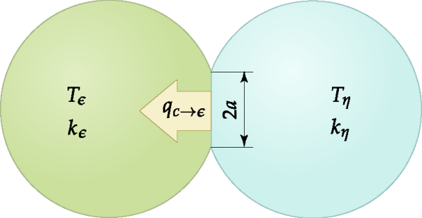
a is the radius of the contact surface, which is depicted
schematically in Figure 2.6: Heat transfer between two colliding particles.. In order to determine the value of the contact radius, Batchelor &
O'Brien considered the Hertz theory, according to which we have:
(2–59) |
where:
is the instantaneous normal contact force between the two particles or the particle and the wall.
is the equivalent radius, defined in Equation 2–15.
is the effective Young's modulus, defined in Equation 2–14.
Equation 2–58 and Equation 2–59 are used in Rocky at
particle-boundary contacts as well, considering the appropriate definitions for the involved
parameters. Regarding the equivalent thermal conductivity used in Equation 2–58, as the thermal conductivities of the particle and its neighbor can be different in a general case, in Rocky it is
defined as the harmonic mean:
(2–60) |
where and
are the thermal conductivities of the two contacting entities.
The heat transfer rate between two elements of a flexible particle connected by a virtual joint is modeled in Rocky as:
(2–61) |
where and
are the temperatures of the two connected elements, while
is the joint equivalent conductance, given by:
(2–62) |
where Hp and
are the partial thermal conductances at each side of the joint,
approximated respectively as:
(2–63) |
(2–64) |
In these expressions, and
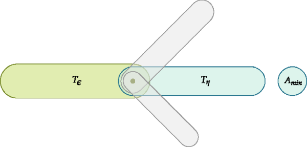
are the distances from the centroid of the joint to the centroid of the
respective element, as shown in Figure 2.7: Heat transfer between two elements in a flexible fiber. , in a flexible fiber example.
Additionally,
is the thermal conductivity of the joint, defined as:
(2–65) |
where is the thermal conductivity of the particle's material and
is a user input parameter, listed in the Rocky UI on the
Composition sub-tab for the Particle set as
Conductivity Ratio. This parameter allows users to make
fine adjustments to the joint's thermal conductivity without modifying the particle's
thermal conductivity, which is used in the calculation of the contact conductance as well.
Allowed values for the conductivity ratio are in the range from 0.01 to 100.
In Equation 2–63 and Equation 2–64, is the effective area of the joint. In most cases,
will be the area of the section that connects two elements. For straight
fibers, it will be the area of the circular section of the cylindrical part of the elements.
For shells, it will be the area of a rectangular face connecting two prismatic elements. For
solid particles, it will be the area of the triangular face connecting two tetrahedral
elements.
The case of multi-branched custom fibers is the one that poses certain difficulties for
defining . The main difficulty is that several sphero-cylinder elements can meet at
a given point, each one having a different diameter, as depicted in the example of Figure 2.8: Example of a multi-branched custom fiber. In this case, the number of coincident
elements
=4. For the joint between the green and blue elements,
is the cross sectional area of the blue element (the one with the
smallest diameter).. As an
element may be connected to more than one element at one of its ends, this reduces the
effective area for transferring heat to any of the connected elements at that place.
Therefore, we define the following effective area for those cases:
(2–66) |
where is the smallest cross sectional area between the two elements connected by
the given joint, while
is the number of fiber elements that meet at the same point were that
joint is located.
Figure 2.8: Example of a multi-branched custom fiber. In this case, the number of coincident
elements =4. For the joint between the green and blue elements,
is the cross sectional area of the blue element (the one with the
smallest diameter).

Decreasing stiffness in order to speed up a simulation has the undesired side effect of abnormally increasing the predicted heat exchange. When the contact stiffness is decreased using the Numerical Softening Factor , the contact area and the collision time are increased, both causing an artificial rise of the heat transferred through a contact. In order to counteract those adverse effects, Rocky includes two correction strategies proposed initially by Morris et al..
The correction is valid for static systems. When enabled by the user in the Thermal tab of the Physics panel, this correction model replaces the reduced Young's modulus of particles or boundaries by the actual values specified by the user for the respective materials, when calculating the contact radius using .
The correction is indicated for simulations with non-resting particles. This model
extends by also applying a further correction factor to the area-corrected contact radius during collisions in order to
mitigate the adverse thermal effect caused by artificially longer contact times between
softened particles.
This model was deduced by considering the theoretical exchanged heat rate during a collision between two particles for the actual and softened cases, and provides the following correction factor for the collision time:
(2–67) |
where:
is the collision time between the softened particles.
is the collision time between the actual particles.
The correction factor also equals to the ratio of the actual and area-corrected thermal contact
conductances between the colliding particles. Therefore for a Hertzian collision model it
can also be interpreted as a multiplier to the instantaneous, area-corrected contact radius
between softened particles during the simulation.
Still considering a Hertzian collision model, can be simplified to:
(2–68) |
where is the Numerical Softening Factor of the
simulation. Thermal conduction correction models is employed by Rocky when the Morris et al. Area+Time correction model is enabled by the user.


