


Rocky can be used also as a tool for the prediction of abrasive wear of solid surfaces due to the action of impacting particles. The wear model implemented in Rocky is based on Archard's wear law [27]. This phenomenological law relates the volume loss of material to the work done by the frictional forces on the surface of the material. Archard?s law is usually expressed as [28]:
 | (2–51) |
where:
 is the total volume of material worn from the surface.
  is the work done by the tangential forces over the surface.
  H is the hardness of the material subjected to wear.
  k is a dimensionless empirical constant.
For the purpose of implementation in Rocky, Archard's law is considered in the incremental form:
 | (2–52) |
where:
 is the volume of material worn during a simulation timestep.
  is the tangential or shear work done by the contact forces over the
boundaries during a timestep, at particle-to-boundary contacts.
is the tangential or shear work done by the contact forces over the
boundaries during a timestep, at particle-to-boundary contacts.  is a constant provided by the user. In Rocky, every imported boundary in
a problem can be defined with a different value of the constant
is a constant provided by the user. In Rocky, every imported boundary in
a problem can be defined with a different value of the constant  , listed in the UI as
Volume/Shear Work Ratio.
, listed in the UI as
Volume/Shear Work Ratio.
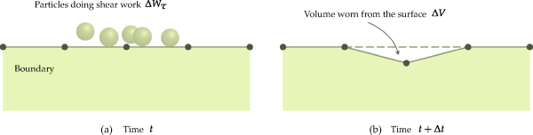
Figure 2.5: Schematic depiction of the wear of a surface. illustrates schematically the application of Equation 2–52 in Rocky. Since all boundaries in Rocky are defined as triangulated
surfaces, the effect of removing the volume  is achieved by displacing their vertices inwards. The distance that every
vertex is displaced is calculated in order to make the volume variation equal to the value of
is achieved by displacing their vertices inwards. The distance that every
vertex is displaced is calculated in order to make the volume variation equal to the value of  calculated with Equation 2–52. It is worth noting that during this process the topology
of the boundary triangulation is maintained unchanged. Because of this, in order to capture
adequately geometry changes, it is desirable that regions expected to suffer wear present
triangulations sufficiently refined.
calculated with Equation 2–52. It is worth noting that during this process the topology
of the boundary triangulation is maintained unchanged. Because of this, in order to capture
adequately geometry changes, it is desirable that regions expected to suffer wear present
triangulations sufficiently refined.
The tangential work done by the particles colliding with a boundary is computed triangle by triangle. Vertices adjacent to triangles that receive more shear work will displace more and, consequently, these regions will show more wear in a simulation. The tangential work per triangle is calculated by adding the tangential work contributions of all collisions occurring in a triangle during a simulation timestep. Conventionally, the work that produces wear over a boundary at a single particle-to-boundary contact is considered to be one half of the total work done by the respective tangential contact force. That is:
 | (2–53) |
where:
 is the tangential component of the contact force, calculated by one of
the Rocky's tangential force models.
is the tangential component of the contact force, calculated by one of
the Rocky's tangential force models.  is the sliding distance computed during a simulation timestep,
  . The sliding distance is the relative displacement parallel to the
tangential plane, at a particle-to-boundary contact.
. The sliding distance is the relative displacement parallel to the
tangential plane, at a particle-to-boundary contact.
In general, the actual period of life of wear in industrial processes is much longer than what is usually reasonable to simulate using DEM. This problem can be circumvented by shortening the simulation time while increasing the wear rate C several orders of magnitude. A suitable value of C can be determined by following two heuristic rules [28]:
C must satisfy the constraint of proportionality of Equation 2–52. In other words, increasing C by a factor and reducing the simulation time by the same factor must preserve the wear characteristics.
The entire simulation time must be sufficiently long, so the statistical variance associated with discrete events is small in the DEM output data.
Both rules are violated when extremely large values of C are used, producing fast changes in geometry that strongly disturb the motion of particles.