


For the momentum transfer using CGM, the focus is to respect the first three
constraints listed in the previous section. The first two define that the terminal velocity of
the particles must be kept the same on the scaled-up system. This is important in fluidized
bed cases, for example, where the terminal velocity has an important role on the phenomena.
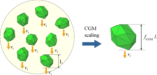
Figure 5.1: Terminal velocity conservation
when using CGM scale-up. shows the idea of the conservation of terminal
velocity on the scaled-up system. It shows a collection of small (original) particles falling
on a stagnant fluid that is replaced by a larger parcel (scaled-up particle), in which the CGM
upscaling imposes that the terminal velocity of the larger parcel is equal to the terminal
velocity of the original particles. In this example  .
.
The third constraint is related to the pressure drop of the fluid flow when crossing a bed of static particles.
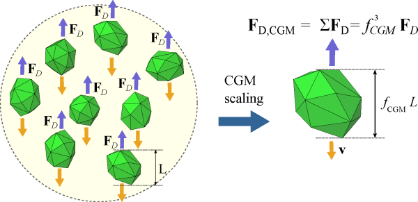
To satisfy this condition, the fluid forces over the parcel should be equal to the sum
of the fluid forces on each one of the original particles, which is approximated by the force
on a single particle times the number of particles the parcel represents, given by
 . Figure 5.2: Fluid force on a CGM parcel
is equal to the sum of the forces over the
original particles. shows the fluid force acting over the
parcel given as the sum of the fluid forces acting over all the original particles it
represents. In this example
. Figure 5.2: Fluid force on a CGM parcel
is equal to the sum of the forces over the
original particles. shows the fluid force acting over the
parcel given as the sum of the fluid forces acting over all the original particles it
represents. In this example .
.
Figure 5.2: Fluid force on a CGM parcel is equal to the sum of the forces over the original particles.
No correction is needed for the pressure-gradient force given by Equation 3–4 as the volume of the parcel is already equal to
 times the volume of one of the original particles.
For the drag force, changes need to be applied to Equation 3–5 to satisfy the constraints. As the area of the parcel,
 is equal to
  , just a single scale-factor needs to be multiplied on the equation to
reach the total
, just a single scale-factor needs to be multiplied on the equation to
reach the total  factor needed. The drag force calculation when using the CGM model is
given by Equation 5–1.
factor needed. The drag force calculation when using the CGM model is
given by Equation 5–1.
 | (5–1) |
The the drag coefficient,  , used on Equation 5–1 also needs to be corrected as
the drag coefficient calculated for the parcel has to have the same value as for a single
original particle in order to scale the drag force correctly. Inasmuch as the drag
coefficient is usually a function of the Reynolds number and the volume fraction of
particles, these two numbers must be kept same as for the original system for the sake of
obtaining the same drag coefficient.
, used on Equation 5–1 also needs to be corrected as
the drag coefficient calculated for the parcel has to have the same value as for a single
original particle in order to scale the drag force correctly. Inasmuch as the drag
coefficient is usually a function of the Reynolds number and the volume fraction of
particles, these two numbers must be kept same as for the original system for the sake of
obtaining the same drag coefficient.
The volume of the particles is kept the same on scaling-up, so there is no need to
change the volume fraction calculation. As the scaled particle size is used for the parcel
Reynolds number calculation, the fluid viscosity,  , is also scaled with
  with the aim of keeping the same Reynolds number for the scaled parcel and
the original particle. The corrected Reynolds number equation is shown in Equation 5–2.
with the aim of keeping the same Reynolds number for the scaled parcel and
the original particle. The corrected Reynolds number equation is shown in Equation 5–2.
 | (5–2) |
No correction is needed for the turbulent dispersion force, which is computed as described on section Turbulent dispersion force.
The virtual mass force, calculated using Equation 3–64 also does not need any modifications. It scales with the particle volume and its coefficient depends only on the particles? volume fraction.