The Schiller & Naumann drag correlation for spherical particles provides the drag coefficient for with a maximum deviation of 5% in relation to experimental data [41]. The standard version of the correlation is given by [42]:

(3–7)

A modification commonly used for inclusion of drag inertial range [42], [43], [44] is given by:

(3–8)

The modified version of this drag law is implemented in Rocky DEM-CFD coupling, being the recommended drag law to be used for simulations with spherical particles.

The DallaValle drag law [45] also provides the drag coefficient for spherical particles. Its validity range is up to and its main difference to the modified Schiller & Naumann correlation is that it is a continuous function. The DallaValle correlation is defined by:

(3–9)

Morsi and Alexander [46] describe a theoretical investigation into the motion of a spherical particle subject to (i) a one-dimensional fluid flow, (ii) an uniform two-dimensional fluid flow about a circular cylinder, and (iii) the fluid flow caused by a lifting aerofoil section. In all three cases the drag of the particle is assumed to vary only with the Reynolds number, and the authors derived the following analytical approximation for the drag coefficient:

(3–10)

where and are constants that the user can set. In Rocky, these correspond to parameters and available in the Fluent Two-Way Coupling settings when Morsi & Alexander is selected as the Drag Law and Use Defined Constants checkbox is enabled under the Morsi & Alexander section.

Based on experimental data, Morsi & Alexander (1972) also suggest sets of values for the constants of equation Equation 3–10 according to several ranges of , as listed in Table 3.1:  Values of constants according to ranges of the Reynolds number as implemented in Rocky. . When Use Defined Constants checkbox is not enabled under the Morsi and Alexander section, Rocky employs the values of Table 3.1:  Values of constants according to ranges of the Reynolds number as implemented in Rocky. for the constants and instead of the user-defined values.

Table 3.1: Values of constants according to ranges of the Reynolds number as implemented in Rocky.

	24.0	0	0
	22.73	0.0903	3.69
	29.1667	-3.8889	1.222
	46.5	-116.67	0.6167
	98.33	-2778	0.3644
	148.62	-4.75x104	0.357
	-490.546	57.87x104	0.46
	-1662.5	5.4167x106	0.5191

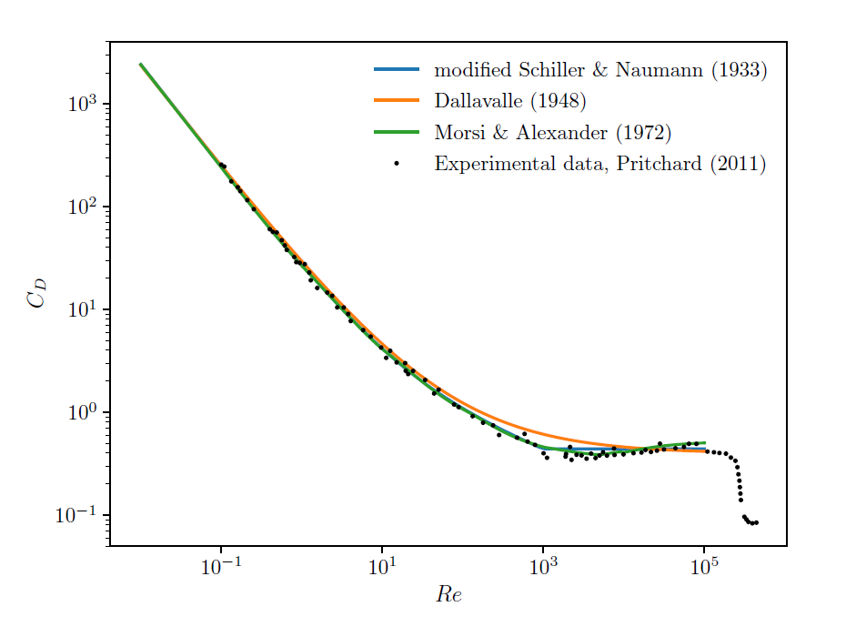
Figure 3.1: Comparison of single particle drag laws for dilute flows to experimental data. compares the drag coefficient obtained using equations (Equation 3–8), (Equation 3–9) and (Equation 3–10) to experimental data for spherical particles. It can be seen that the modified version of Schiller & Naumann drag correlation, the DallaValle correlation and the Morsi & Alexander correlation all fit very well into the spherical experimental data.

Figure 3.1: Comparison of single particle drag laws for dilute flows to experimental data.

Haider & Levenspiel [47] compiled drag coefficient and terminal velocity experimental data for spherical and non-spherical particles. Then, they developed explicit expressions for both types of particles. For spherical particles, the correlation coefficients have fixed values, whereas for non-spherical values they are dependent on the sphericity, which is defined below.

The unified correlation for both types of particles is given by:

(3–11)

For spherical particles, the values of the coefficients in this correlation are:

(3–12)

On the other hand, for non-spherical particles, they are given by the expressions:

(3–13)

where is the particles sphericity, defined as:

(3–14)

where is the surface area of a sphere having the same volume as the particle and is the actual surface area of the particle.

As an illustration of the accuracy of this correlation, presents the comparison of Equation 3–11 with experimental data for spherical and distinct types of non-spherical particles, all with different values of sphericity.

The Haider & Levenspiel drag law the recommended drag law for isometric non-spherical particles and for non-isometric non-spherical particles tolerating some loss of accuracy. The particle sphericity is automatically calculated by Rocky based on the particles shape and size.

Ganser [48] showed that both Stokes shape factor and Newtons shape factor are important for the prediction of drag. Stokes shape factor is defined as the ratio between the drag coefficient of a spherical particle and the drag coefficient for a particle with an arbitrary shape, both in Stokes flow . Newtons shape factor is defined as the ratio between the drag coefficient of a particle with an arbitrary shape and the drag coefficient of a spherical particle, both in .

Thereby, Ganser developed a simplified drag equation that is a function only of the generalized Reynolds number . This equation, applicable to all shapes and valid for is the following:

(3–15)

The suggested expressions of and for isometric and non-isometric particles are, respectively, the following:

(3–16)

(3–17)

where is the diameter of a spherical particle with the same projected area of the actual particle in the direction of the flow, and is the diameter of a spherical particle with the same volume of the actual particle, and is the diameter of the container.

This correlation calculates both the Stokes and Newton parameters, considering the effects of shape and alignment of the particle with the flow field to compute the drag coefficient. This is a more accurate (but also more computationally expensive) option.

The Marheineke and Wegener drag law [49] is applied exclusively to particles based on the sphero-cylinder shape, i.e., straight and custom fibers, both rigid and flexible. Unlike other drag laws available in Rocky, the drag law is not based on Equation 3–5 , because in its formulation it is necessary to consider separately the normal and tangential components of the drag in relation to the cylinder axis.

Let's consider the sphero-cylinder shown in Figure 3.2: Schematic depiction of some parameters considered in the drag law., which can be either a whole sphero-cylinder particle, a segment of a rigid custom fiber, or an element of a flexible fiber (straight or custom). The relevant geometric parameters are the diameter , the length , and the tangential unit vector , which is a unit vector parallel to the sphero-cylinder axis.

Figure 3.2: Schematic depiction of some parameters considered in the drag law.

For application in the formulation of the drag law, the relative velocity of the flow in relation to the sphero-cylinder is defined as:

(3–18)

where is the unperturbed flow velocity, while is the velocity of the geometric center of the sphero-cylinder. The tangential and normal components of this velocity are given, respectively, by:

(3–19)

(3–20)

The tangential component is parallel to the sphero-cylinder axis, while the normal component is parallel to a plane N, orthogonal to that axis. The unit vector in the normal direction will be given by:

(3–21)

Marheineke and Wegener proved the so-called independence principle for the stationary flow around a circular cylinder [49], which states that the normal component of the drag force is independent of the tangential velocity, while the tangential component of the drag force varies linearly with the tangential velocity. This allowed them to formulate the drag force per unit length over an infinite circular cylinder as:

(3–22)

where and are the drag coefficients for the normal and tangential directions, respectively. Both coefficients are functions of the Reynolds number based on the normal component of the velocity, defined as:

(3–23)

Marheineke and Wegener arranged several correlations from other authors as continuously differentiable piecewise expressions for the drag coefficients, each one valid for a specific flow regime. Some of those correlations were obtained using analytical methods, while others are based on results from numerical simulations or on heuristic arguments. In order to write the piecewise expressions in a unified way, it is convenient to define the so-called resistance coefficients:

(3–24)

Introducing them equation Equation 3–22, further reduces to:

(3–25)

The correlations provided by Marheineke and Wegener can be then written as:

(3–26)

The function valid for the is given by:

(3–27)

while the one for is defined as:

(3–28)

Similarly, the function for the normal direction is defined by the expression:

(3–29)

while the equivalent expression for the tangential direction is:

(3–30)

where the parameter is defined as:

(3–31)

The values of the coefficients for the correlations valid for are listed on Table 3.2:  Coefficient values for the correlations (valid on ). On the other hand, the coefficients for the correlations valid for are defined in a way that the resistance coefficients converge asymptotically to the values predicted by the Stokes theory for slender bodies, as . Those values are given by:

(3–32)

(3–33)

Table 3.2: Coefficient values for the correlations (valid on )

0	1.6911	1.1552
1
2
3

where is the slenderness ratio, defined as:

(3–34)

The coefficients that lead to a smooth transition between the portions valid on and the asymptotic values for are the following:

(3–35)

Finally, the position of the transition point depends also on the slenderness ratio through the value of :

(3–36)

Marheineke and Wegener point out that in order to locate the transition point in the low Reynolds number regime, the condition must be fulfilled. This implies that the previous equations are valid only for .

As an illustration, Figure 3.3: Drag resistance in the normal direction, according to the drag law. and Figure 3.4: Drag resistance in the tangential direction, according to the drag law. show plots of for the normal and tangential directions, respectively. In those plots, 4 possible curves are shown in the low Reynolds number regime, for 4 different values of the slenderness ratio.

Figure 3.3: Drag resistance in the normal direction, according to the drag law.

Figure 3.4: Drag resistance in the tangential direction, according to the drag law.

For a relatively low particle concentration (), Wen and Yu [50] developed a drag correlation based on a series of experiments on fluidized beds conducted by Gidaspow [51] . This correlation is presented in terms of a correction (based on fluid volume fraction) of the Schiller & Naumann correlation, using a superficial velocity relative to the particles Reynolds number. The corresponding mathematical expression is [43]:

(3–37)

Ergun [52] studied the pressure losses accompanying the flow of fluids through columns packed with granular material, and found that they are caused by simultaneous kinetic and viscous energy losses according to:

(3–38)

where is the pressure loss suffered by a fluid that flows though a bed of granular material with height , is the superficial relative velocity of the fluid in the direction of the flow and is the effective diameter of the particles of the bed.

Equation 3–38 conforms well to relatively high particle concentrations () up to the maximum packing limit (usually 60 to 70%). It also applies to many types of fluid flow through packed arrangements up to the minimum fluidization condition [52], particularly: gas flow through crushed porous solids, fluid flow through beds of nonporous solids, and fluid flow through solids having uniform geometric shapes.

Some authors [51] and [42] assume the effective diameter in Equation 3–38 as:

(3–39)

Where is the particle sphericity according to Equation 3–14 . Assuming a uniform flow of a weightless gas through a fixed homogeneous bed of spherical particles and considering , the Ergun drag coefficient is deduced from Equation 2–6, Equation 3–38 and Equation 3–39 as:

(3–40)

Gidaspow, Bezburuah & Ding [53] have developed a simple connection between the Wen & Yu and Ergun correlations to represent the complete range of solids volume fraction in a single drag law, by simply applying each law over its valid range. The Gidaspow, Bezburuah & Ding correlation is then given by:

(3–41)

The Gidaspow, Bezburuah & Ding drag correlation covers the entire range of solids (particle phase) volume fraction (from 0 up to the maximum packing limit) but presents a discontinuity at the point . To make the transition between the Wen & Yu and Ergun correlations in a smoother way, Huilin & Gidazpow [37] have applied a blending function to promote the connection based on the fluid volume fraction. The final drag correlation is given by:

(3–42)

The blending parameter is defined as a function of the fluid volume fraction, , given by:

(3–43)

Using experimental data, correlations from previous works and analytical results, Di Felice [36] derived a correction function for the DallaValle (1948) single particle drag coefficient in order to consider the case of dense particle flows. The correlation is given by:

(3–44)

where is the drag coefficient for a single particle, also calculated using the particles Reynolds number based on the superficial relative velocity.

The exponent in Equation 3–44 is calculated by means of:

(3–45)

Using previous studies on the relationship of the terminal velocity of isolated particles with the hindered terminal velocity of concentrated particles, Syamlal and O'Brien [35] [34] originally defined a drag coefficient formula for dense particle flows. The formula reduces to the DallaValle (1948) single-particle drag coefficient when the fluid volume fraction is equal to one.

The authors showed that terminal settling conditions estimated by the formula compares well with experimental data [35] for Reynolds numbers greater than 10. For smaller Reynolds numbers, however, Syamlal and O'Brien (1987) tends to over-predict the Reynolds number.

The parameterized Syamlal and O'Brien model implemented in Rocky is an enhancement of Syamlal and O'Brien (1987) in which two constants of the model are replaced by user-defined parameters. When these parameters are adjusted based on the fluid properties and the expected minimum fluidization velocity, the parameterized Syamlal and O'Brien model may overcome the tendency of Syamlal and O'Brien (1987) to over-predict bed expansion [44].

The Syamlal and O'Brien drag coefficient is defined as:

(3–46)

where is the single particle drag coefficient, is the fluid volume fraction and , the terminal velocity ratio.

In Equation 3–46, the single particle drag coefficient has the same formula as the one proposed by DallaValle in but, instead of using the particle Reynolds number directly on the correlation, the ratio of the particle Reynolds number over the terminal velocity ratio is applied:

(3–47)

The terminal velocity ratio is the ratio of the settling fluid velocity of a dense system to that of a single particle and is computed as:

(3–48)

In Equation 3–48, A and B are functions of the fluid volume fraction:

(3–49)

(3–50)

where and are parameters of the model that must be defined by the user. In Rocky, these are accessible through inputs and in the Fluent Two-Way Coupling settings when Syamlal and O'Brien is selected as the drag law.

The parameters and are commonly used to adjust the minimum fluidization velocity at the minimum fluidization condition in simulations of fluidized beds. If the user desires B to be continuous at in Equation 3–50, the following relationship between and must be respected:

(3–51)

The combination of the Ergun and Wen & Yu equations is a widely used drag model, where the latter law should be automatically selected when the local porosity exceeds 0.8, as recommended by Gera et al [33]. and Kuipers et al. [32]. However, Koch and Hill [31] described large discrepancies of this drag model combination after performing Lattice Boltzmann (LBM) simulations. This issue occurs especially for low porosities (below 0.8) and at higher Reynolds numbers . Therefore the Hill-Koch drag correlation is a discontinuous function that switches the correlation depending on the porosity field () as written below:

(3–52)

where is the drag coefficient, and and are coefficients that depend on the porosity given by:

(3–53)

(3–54)

where the threshold porosity transition in the Hill-Koch 2001 model is chosen to be 0.6.

One of the problems with the Hill-Koch 2001 correlation is the discontinuity regarding the porosity field . In 2006, Benyahia et al. [30] proposed an extension of the Hill-Koch model such that the drag coefficient is described by a continuous function of the porosity field and the relative Reynolds number . The numerical experiments conducted by Benyahia et al. makes the extended Hill-Koch-Ladd 2006 law valid for large ranges of and , especially in fluid flow regimes found commonly in fixed-bed reactors. The model switches between optimal representation of drag correlation; however, due its construction, it does not present abrupt transitions in the drag coefficient calculation. For those cases, the original Koch and Hill [29] correlation is a more appropriate choice. The drag coefficient is calculated by the following expression:

(3–55)

where the function changes according to Reynolds and porosity :

(3–56)

where the coefficients and the Reynolds criteria limits and are given by:

(3–57)

(3–58)

(3–59)

(3–60)

(3–61)

(3–62)

(3–63)

where is the solid volume fraction and is a weight function required by and .

A comparison among all drag laws for dense flows is presented in Figure 3.5: Comparison of dense flow drag laws for for a constant fluid volume fraction of . At this value of the volume fraction all correlations seem to match, but one must consider the differences when varying the fluid volume fraction as well.

Figure 3.5: Comparison of dense flow drag laws for

Figure 3.6: Comparison of dense flow drag laws for

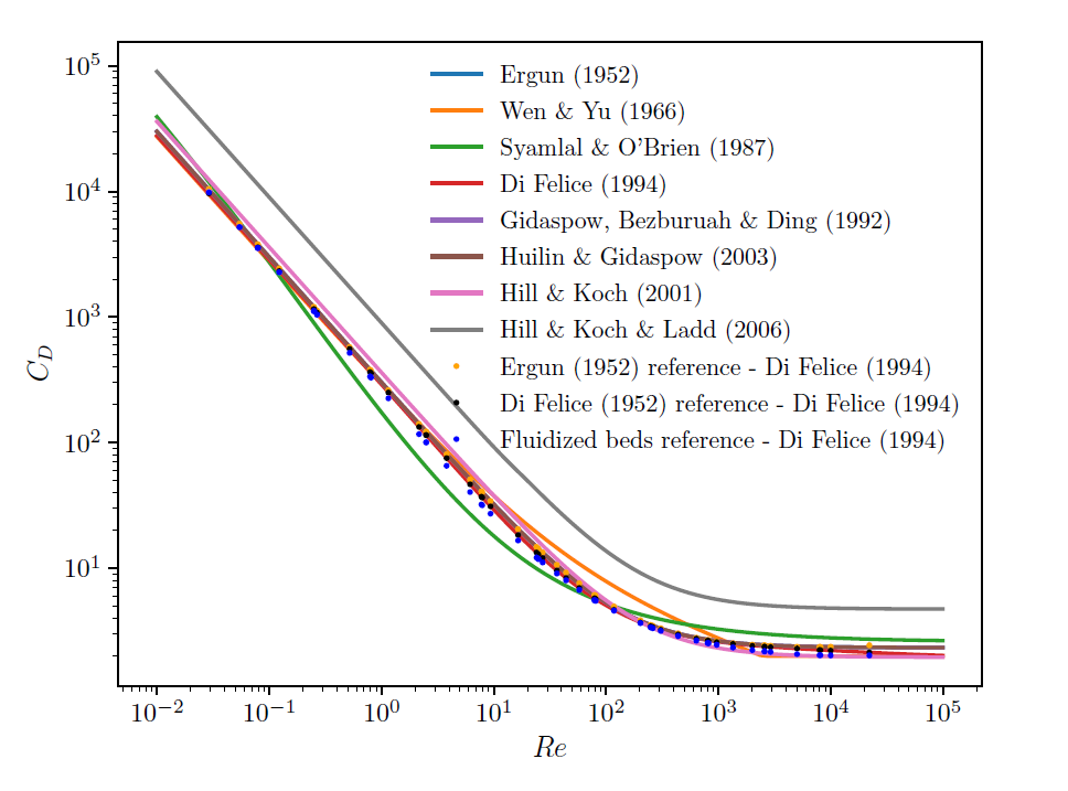
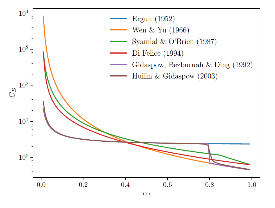
Figure 3.6: Comparison of dense flow drag laws for shows the variation of these same laws for a fixed and a varying fluid volume fraction. The variances are significant and may generate considerable differences in overall particle-fluid interactions during simulations.