The Parameter Study will be performed through a series of runs, where a separate subdirectory for each run will be created beneath the Project Working Directory. This Run Working DIrectory contains a copy of all needed input files and the output files generated by the run. The Solution Harvester is invoked during post-processing of the Parameter Study. The Harvester serves to parse the solution files generated for each run and creates a merged solution set that can easily be analyzed using the visualization options of the Post-Processor.
Here, we use the project closed_homogeneous__transient.ckprj as an example of running a Parameter Study.
You can run the Parameter Study using the following steps:
Open the project closed_homogeneous__transient.ckprj and pre-process its chemistry set.
Follow the steps listed in Setting up a Single Parameter Variation and Setting up Multiple Parameter Variations to set up parameter variations for temperature and pressure using the Superimpose all parameter variations mode.
Follow the steps listed in Setting up a Parameter Study to set up parameter variations for activation energy of the gas-phase reaction O + H2 = OH + H to have six points from 6290.0 to 6490.0 using the Superimpose all parameter variations mode.
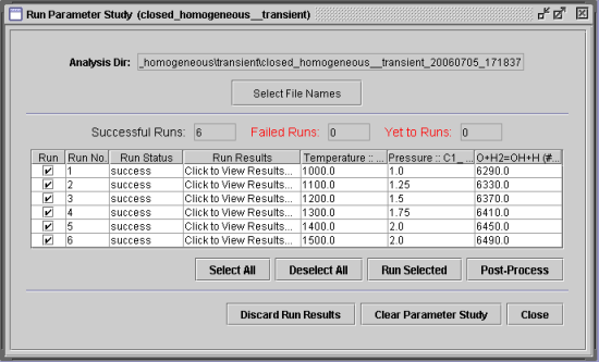
If you want to see the details regarding the Parameter Study runs, click the Display Detail button and the Parameter Study panel will show up in the interface.
Click the Begin button to run the Parameter Study Facility. It will create a new directory, closed_homogeneous__transient_########_######, in your Project Working Directory, where the #s in the name are replaced by a unique date- and time-based tag. Each run creates a separate run directory named by the run number within this directory.
During the runs, a Monitor Project Run panel will open in the interface. This panel displays the current progress of the parameter study. You can click the Interrupt Jobs button to skip the runs that have not started yet. You can also open this panel at any time by double-clicking on the Monitor Project Run node of the project tree.
When all the runs are complete, you will see the overall status displayed at the top of the Running Parameter Study panel as well as the Run Status column. To view the diagnostic output file and log file of each run, you can click the View Results… pull-down list in the Run Results column.
Double-click the Analyze Results node in the project tree. An Analyze Results panel will open in the interface.
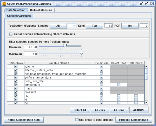
Click the Begin Analysis button and a Select Post-Processing Variables panel, as shown in Figure 2.7: closed_homogeneous__transient.ckprj - Select Post-Processing Variables, will open to allow you to select solution parameters to plot in the Ansys Chemkin Post-Processor. You can select solution sets (if available), select species and variables, apply various filters and options, and set the units of measure, as discussed in Properties Available for Use in the Parameter Study Facility.
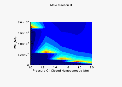
When you are done selecting variables and units, click the Process Solution Data button. A Monitor Project Run panel will open to display the progress of post-processing jobs. After all the post-processing jobs are finished, the data harvester will parse through the solution files over all runs to create a merged solution set and the Ansys Chemkin Post-Processor will be invoked automatically to allow you to graphically visualize all of the solution data. For example, you can create a contour plot from the contour set of CKSoln_vs_parameter.csv using Pressure C1 Closed Homogeneous as the X variable, Time as the Y variable, and Mole Fraction H as the Z variable, as seen in Figure 2.8: closed_homogeneous__transient.ckprj - Contour Plot for Mole Fraction H.