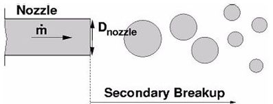
This is one of the simplest and most popular approaches to define the injection conditions of droplets. In this approach, it is assumed that a detailed description of the atomization and breakup processes within the primary breakup zone of the spray is not required. Spherical droplets with uniform size, , are injected that are subject to aerodynamic induced secondary breakup.

Assuming non-cavitating flow inside the nozzle, it is possible to compute the droplet injection velocity by conservation of mass:

(6–107)

is the nozzle cross-section and the mass flow rate injected through the nozzle.

The spray angle is either known or can be determined from empirical correlations. The blob method does not require any special settings and it is the default injection approach in CFX.

Figure 6.1: Blob Method

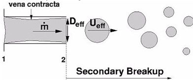
Kuensberg et al. [110] have suggested an enhanced version of the blob-method. Similar to the blob-method, it is assumed that the atomization processes need not be resolved in detail. Contrary to the standard blob-method, this method enables you to calculate an effective injection velocity and an effective injection particle diameter taking into account the reduction of the nozzle cross-section due to cavitation.

During the injection process, the model determines if the flow inside the nozzle is cavitating or not and dynamically changes the injection particle diameter and the particle injection velocity. The decision, whether the flow is cavitating or not, is based on the value of the static pressure at the vena contracta, , that is compared to the vapor pressure, .

(6–108)

with:

(6–109)

is the coefficient of contraction that depends on nozzle geometry factor, such as nozzle length versus nozzle diameter or the nozzle entrance sharpness [114].

If is higher than the vapor pressure, , the flow remains in the liquid phase and the injection velocity is set equal to .

(6–110)

The initial droplet diameter is equal to the nozzle diameter, .

However, if is lower than , it is assumed that the flow inside the nozzle is cavitating and the new effective injection velocity, , and injection diameter, , are computed from a momentum balance from the vena contracta to the nozzle exit (2):

(6–111)

and:

(6–112)

with:

(6–113)

Figure 6.2: Enhanced-blob Method

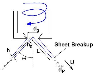
The LISA (Linearized Instability Sheet Atomization) model is able to simulate the effects of primary breakup in pressure-swirl atomizers as described in this section and presented in detail by Senecal et al. [126].

In direct-injection spark ignition engines, pressure swirl atomizers are often used in order to establish hollow cone sprays. These sprays are typically characterized by high atomization efficiencies. With pressure swirl injectors, the fuel is set into a rotational motion and the resulting centrifugal forces lead to a formation of a thin liquid film along the injector walls, surrounding an air core at the center of the injector. Outside the injection nozzle, the tangential motion of the fuel is transformed into a radial component and a liquid sheet is formed. This sheet is subject to aerodynamic instabilities that cause it to break up into ligaments.

Figure 6.3: Pressure Swirl Atomizer

Within the LISA model, the injection process is divided into two stages:

 

6.5.1.3.1. Film Formation

Due to the centrifugal motion of the liquid inside the injector, a liquid film along the injector walls is formed. The film thickness, , at the injector exit can be expressed by the following relation:

(6–114)

where is the mass flow rate through the injector, is the particle density, and is the injector exit diameter. The quantity is the axial velocity component of the film at the injector exit and depends on internal details of the injector. In CFX, is calculated using the approach of Han et al. [127]. It is assumed that the total velocity, , is related to the injector pressure by the following relation:

(6–115)

where is the pressure difference across the injector and is the discharge coefficient, which is computed from:

(6–116)

Assuming that is known, the total injection velocity can be computed from Equation 6–115. The axial film velocity component, , is then derived from:

(6–117)

where is the spray angle, which is assumed to be known. At this point, the thickness, , and axial velocity component of the liquid film are known at the injector exit. Note that the computed film thickness, , will be equal to half the injector nozzle diameter if the discharge coefficient, , is larger than 0.7. The tangential component of velocity () is assumed to be equal to the radial velocity component of the liquid sheet downstream of the nozzle exit. The axial component of velocity is assumed to remain constant.

 

6.5.1.3.2. Sheet Breakup and Atomization

After the liquid film has left the injector nozzle, it is subject to aerodynamic instabilities that cause it to break up into ligaments. The theoretical development of the model is given in detail by Senecal et al. [126] and is only briefly repeated here.

The model assumes that a two-dimensional, viscous, incompressible liquid sheet of thickness moves with velocity through a quiescent, inviscid, incompressible gas medium. A spectrum of infinitesimal disturbances is imposed on the initially steady motion, and is given in terms of the wave amplitude, , as:

(6–118)

where is the initial wave amplitude, is the wave number, is the complex growth rate, is the streamwise film coordinate, and is the time. The most unstable disturbance, , has the largest value of and is assumed to be responsible for sheet breakup.

As derived by Senecal et al. [126], can be computed by finding the maximum of the following equation:

(6–119)

here , that is, the ratio of local gas density to particle densities , and is the surface tension coefficient. Once is known, the breakup length, , and the breakup time, , are given by:

(6–120)

(6–121)

where is the critical wave amplitude at breakup and is an empirical sheet constant with a default value of 12.

The unknown diameter, , of the ligaments at the breakup point is obtained from a mass balance. For wavelengths that are long compared to the sheet thickness (; here the Weber Number, , is based on half the film thickness and the gas density), is given by:

(6–122)

using the long wave ligament factor, , of 8.0 (default) and is the wave number corresponding to the maximum growth rate, .

For wavelengths that are short compared to the sheet thickness, is given by:

(6–123)

In this case, the short wave ligament factor, , of 16.0 (default) is used and is given by:

(6–124)

The most probable droplet diameter that is formed from the ligaments is determined from:

(6–125)

using the droplet diameter size factor of 1.88 (default) and is the particle Ohnesorge number that is defined as:

(6–126)

where is the Weber Number based on half the film thickness and the gas density. is the Reynolds Number based on the slip velocity.

This atomization model is based on the modification of the Huh and Gosman model as suggested by Chryssakis (see [155, 156]). It accounts for turbulence induced atomization and can also be used to predict the initial spray angle. The model assumes that turbulent fluctuations within the injected liquid produce initial surface perturbations, which grow exponentially by the aerodynamic induced Kelvin-Helmholtz mechanism and finally form new droplets. The initial turbulent fluctuations at the nozzle exit are estimated from simple overall mass, momentum and energy balances. Droplets are injected with an initial diameter equal to the nozzle diameter, . It is assumed that unstable Kelvin-Helmholtz waves grow on their surfaces, which finally break up the droplet. The effects of turbulence are introduced by assuming, that the atomization length scale, , is proportional to the turbulence length scale and that the atomization time scale, , can be written as a linear combination of the turbulence time scale (from nozzle flow) and the wave growth time scale (external aerodynamic forces). At breakup, child droplets also inherit a velocity component normal to their parents’ velocity direction. This is different to the model suggested by Chryssakis, where child droplets did not get this velocity component.

The initial spray angle is computed from the following relation:

(6–127)

The model does not take effects of cavitation into account, but assumes that the turbulence at the nozzle exit completely represents the influence of the nozzle characteristics on the atomization process.

Primary breakup models are used to determine starting conditions for the droplets that leave the injection nozzle. To accomplish this task, the models use averaged nozzle outlet quantities, such as liquid velocity, turbulent kinetic energy, location and distribution of liquid and gas zones, as input for the calculation of initial droplet diameters, breakup times and droplet injection velocities. Because all detailed information is replaced by quasi 1D data, the following restrictions will apply: