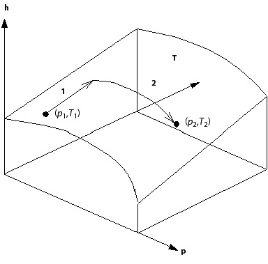
In order to support general properties, which are a function of both temperature and pressure, a table for is generated by integrating Equation 1–8 using the functions supplied for and . The enthalpy table is constructed between the upper and lower bounds of temperature and pressure (using flow solver internal defaults or those supplied by the user). For any general change in conditions from to , the change in enthalpy, , is calculated in two steps: first at constant pressure, and then at constant temperature using Equation 1–9.

(1–9)

To successfully integrate Equation 1–9, the CFX-Solver must be provided thermodynamically consistent values of the equation of state, , and specific heat capacity, . "Thermodynamically consistent" means that the coefficients of the differential terms of Equation 1–7 must satisfy the exact differential property that:

(1–10)

or, in terms of the expressions given in Equation 1–8:

(1–11)

To satisfy in Equation 1–11, variables of the form '<Material Name>.Property Residual' are computed and should resolve to zero.

The equation of state derivative within the second integral of Equation 1–9 is numerically evaluated from the using a two point central difference formula. In addition, the CFX-Solver uses an adaptive number of interpolation points to construct the property table, and bases the number of points on an absolute error tolerance estimated using the enthalpy and entropy derivatives.

In the simplified case where a material has constant and , temperatures can be calculated by integrating a simplified form of the general differential relationship for enthalpy:

(1–13)

which is derived from the full differential form for changes in static enthalpy. The default reference state in the CFX-Solver is and .

The enthalpy change for an ideal gas or CHT solid with specific heat as a function of temperature is defined by:

(1–14)

When the solver calculates static enthalpy, either directly or from total enthalpy, you can back static temperature out of this relationship. When varies with temperature, the CFX-Solver builds an enthalpy table and static temperature is backed out by inverting the table.

To properly handle materials with an equation of state and specific heat that vary as functions of temperature and pressure, the CFX-Solver needs to know enthalpy as a function of temperature and pressure, .

can be provided as a table using, for example, an .rgp file. If a table is not pre-supplied, and the equation of state and specific heat are given by CEL expressions or CEL user functions, the CFX-Solver will calculate by integrating the full differential definition of enthalpy change.

Given the knowledge of and that the CFX-Solver calculates both static enthalpy and static pressure from the flow solution, you can calculate static temperature by inverting the enthalpy table:

(1–15)

In this case, you know , from solving the flow and you calculate by table inversion.

If and are constant, then the total temperature and static temperature are equal because incompressible fluids undergo no temperature change due to addition of kinetic energy. This can be illustrated by starting with the total enthalpy form of the constitutive relation:

(1–16)

and substituting expressions for Static Enthalpy and Total Pressure for an incompressible fluid:

(1–17)

(1–18)

some rearrangement gives the result that:

(1–19)

for this case.

For this case, enthalpy is only a function of temperature and the constitutive relation is:

(1–20)

which, if one substitutes the relation between static and total enthalpy, yields:

(1–21)

The total temperature is evaluated with:

(1–22)

using table inversion to back out the total temperature.

In this case, total temperature is calculated in the exact same way as static temperature except that total enthalpy and total pressure are used as inputs into the enthalpy table:

(1–23)

In this case you know , and you want to calculate , but you do not know . So, before calculating the total temperature, you need to compute total pressure. For details, see Total Pressure.

For details, see Rotating Frame Quantities.

In this case, changes in enthalpy as a function of temperature and pressure are given by:

(1–26)

and when this is substituted into the second law gives the following expression for changes in entropy as a function of temperature only:

(1–27)

which, when integrated, gives an analytic formula for changes in entropy:

(1–28)

For ideal gases changes in entropy are given by the following equation:

(1–29)

which for general functions for the solver computes an entropy table as a function of both temperature and pressure. In the simplified case when is a constant, then an analytic formula is used:

(1–30)

This is the most general case handled by the CFX-Solver. The entropy function, , is calculated by integrating the full differential form for entropy as a function of temperature and pressure. Instead of repetitively performing this integration the CFX-Solver computes a table of values at a number of temperature and pressure points. The points are chosen such that the approximation error for the entropy function is minimized.

The error is estimated using derivatives of entropy with respect to temperature and pressure. Expressions for the derivatives are found by substituting the formula for general enthalpy changes into the second law to get the following expression for changes in entropy with temperature and pressure:

(1–31)

which when compared with the following differential form for changes in entropy:

(1–32)

gives that:

(1–33)

(1–34)

The derivative of entropy with respect to temperature is exactly evaluated, while the derivative with respect to pressure must be computed by numerically differentiating the equation of state. Note that when properties are specified as a function of temperature and pressure using CEL expressions the differential terms in Equation 1–31 must also satisfy the exact differential relationship:

(1–35)

or,

(1–36)

Also, see the previous section on Static Enthalpy for more details.

Unless an externally provided table is supplied, an entropy table is built by using the and functions supplied by you and integrating the general differential form:

(1–37)

To calculate total pressure, you also need to evaluate entropy as a function of enthalpy and pressure, rather than temperature and pressure. For details, see Total Pressure.

The recipe to do this is essentially the same as for the temperature and pressure recipe. First, you start with differential form for :

(1–38)

and comparing this with a slightly rearranged form of the second law:

(1–39)

you get that:

(1–40)

(1–41)

In this case, the entropy derivatives with respect to and can be evaluated from the constitutive relationship (getting from and by table inversion) and the equation of state . Points in the table are evaluated by performing the following integration:

(1–42)

over a range of and , which are determined to minimize the integration error.

For incompressible flows, such as those of liquids and low speed gas flows, the total pressure is given by Bernoulli’s equation:

(1–43)

which is the sum of the static and dynamic pressures.

When the flow is compressible, total pressure is computed by starting with the second law of thermodynamics assuming that fluid state variations are locally isentropic so that you get:

(1–44)

The left hand side of this expression is determined by the constitutive relation and the right hand side by the equation of state. For an ideal gas, the constitutive relation and equation of state are:

(1–45)

(1–46)

which, when substituted into the second law and assuming no entropy variations, gives:

(1–47)

where and are the static and total temperatures respectively (calculation of these quantities was described in two previous sections, Static Temperature and Total Temperature). If is a constant, then the integral can be exactly evaluated, but if varies with temperature, then the integral is numerically evaluated using quadrature. For details, see:

Total pressure calculations in this case are somewhat more involved. You need to calculate total pressure given the static enthalpy and static pressure, which the CFX-Solver solves for. You also want to assume that the local state variations, within a control volume or on a boundary condition, are isentropic.

Given that you know (from integrating the differential form for enthalpy) and , you can compute two entropy functions and . There are two options for generating these functions:

Once you have the table, calculated as described in Entropy, computing total pressure for a single pure component is a relatively trivial procedure:

For details, see Rotating Frame Quantities.

For incompressible flows, the total pressure is defined as:

(1–52)

where is static pressure. The stationary frame total pressure is defined as:

(1–53)

For compressible flows relative total pressure, rotating frame total pressure and stationary frame total pressure are computed in the same manner as in Total Pressure. First you start with the relative total enthalpy, rothalpy and stationary frame total enthalpy:

(1–54)

(1–55)

(1–56)

where is the static enthalpy. In a rotating frame of reference, the CFX-Solver solves for the total enthalpy, , which includes the relative kinetic energy.

If you again assume an ideal gas equation of state with variable specific heat capacity you can compute relative total temperature, total temperature and stationary frame total temperature using:

(1–57)

and:

(1–58)

and:

(1–59)

where all the total temperature quantities are obtained by inverting the enthalpy table. If is constant, then these values are obtained directly from these definitions:

(1–60)

(1–61)

(1–62)

At this point, given , , , and you can compute relative total pressure, total pressure or stationary frame total pressure using the relationship given in the section describing total pressure. For details, see Total Pressure.

The names of the various total enthalpies, temperatures, and pressures when visualizing results in CFD-Post or for use in CEL expressions is as follows.

Table 1.1: Variable naming: Total Enthalpies, Temperatures, and Pressures

Variable	Long Variable Name	Short Variable Name
	Total Enthalpy	htot
	Rothalpy	rothalpy
	Total Enthalpy in Stn Frame	htotstn
	Total Temperature in Rel Frame	Ttotrel
	Total Temperature	Ttot
	Total Temperature in Stn Frame	Ttotstn
	Total Pressure in Rel Frame	ptotrel
	Total Pressure	ptot
	Total Pressure in Stn Frame	ptotstn

The Mach Number and stationary frame Mach numbers are defined as:

(1–63)

(1–64)

where is the local speed of sound.

Rotating and stationary frame total temperature and pressure are calculated the same way as described in Total Temperature and Total Pressure. The only changes in the recipes are that rotating frame total pressure and temperature require rothalpy, , as the starting point and stationary frame total pressure and temperature require stationary frame total enthalpy, .