Cubic equations of state are a convenient means for predicting real fluid behavior. They are highly useful from an engineering standpoint because they generally only require that you know the fluid critical point properties, and for some versions, the acentric factor. These properties are well known for many pure substances or can be estimated if not available. They are called cubic equations of state because, when rearranged as a function volume they are cubic in volume. This means that cubic state equations can be used to predict both liquid and vapor volumes at a given pressure and temperature. Generally the lowest root is the liquid volume and the higher root is the vapor volume.

Four versions of cubic state equations are available: Standard Redlich Kwong, Aungier Redlich Kwong, Soave Redlich Kwong, and Peng Robinson. The Redlich-Kwong equation of state was first published in 1949 [85] and is considered one of the most accurate two-parameter corresponding states equations of state. More recently, Aungier (1995) [96] has modified the Redlich-Kwong equation of state so that it provides much better accuracy near the critical point. The Aungier form of this equation of state is the default cubic equation used by Ansys CFX. The Peng Robinson [157]] and Soave Redlich Kwong equation of state were developed to overcome the shortcomings of the Redlich Kwong equations to accurately predict liquid properties and vapor-liquid equilibrium.

 

1.2.2.3.1.1. Redlich Kwong Models

The Redlich Kwong variants of the cubic equations of state are written as:

(1–96)

where is the specific volume .

 

1.2.2.3.1.1.1. The Standard Redlich Kwong Model

The Standard Redlich Kwong model sets the parameter to zero, and the function to:

(1–97)

where is and

(1–98)

(1–99)

 

1.2.2.3.1.1.2. The Aungier Redlich Kwong Model

The Aungier form differs from the original by a non-zero parameter that is added to improve the behavior of isotherms near the critical point, as well as setting the exponent differently. The parameter in Equation 1–96 is given by:

(1–100)

and the standard Redlich Kwong exponent of is replaced by a general exponent . Optimum values of depend on the pure substance. Aungier (1995) [96] presented values for twelve experimental data sets to which he provided a best fit polynomial for the temperature exponent in terms of the acentric factor, :

(1–101)

 

1.2.2.3.1.1.3. The Soave Redlich Kwong Model

The Soave Redlich Kwong real gas model was originally published by Soave (1972). The model applies to non-polar compounds and improves on the original Redlich Kwong model by generalizing the attraction term to depend on the acentric factor, which accounts for molecules being non-spherical, and accounting for a range of vapor pressure data in the development of the temperature dependency of this parameter.

The Soave Redlich Kwong equation is explicit in pressure, and given by:

(1–102)

where:

(1–103)

as in the original Redlich Kwong equation, and

(1–104)

where:

(1–105)

and the parameter n is computed as a function of the acentric factor, ω:

(1–106)

 

1.2.2.3.1.2. Peng Robinson Model

The Peng Robinson model also gives pressure as a function of temperature and volume:

(1–107)

where:

(1–108)

as in the original Redlich Kwong equation, and

(1–109)

where:

(1–110)

and the parameter n is computed as a function of the acentric factor, ω:

(1–111)

 

1.2.2.3.1.3. Real Gas Constitutive Relations

In order to provide a full description of the gas properties, the flow solver must also calculate enthalpy and entropy. These are evaluated using slight variations on the general relationships for enthalpy and entropy that were presented in the previous section on variable definitions. The variations depend on the zero pressure, ideal gas, specific heat capacity and derivatives of the equation of state. The zero pressure specific heat capacity must be supplied to Ansys CFX while the derivatives are analytically evaluated from Equation 1–96 and Equation 1–107.

Internal energy is calculated as a function of temperature and volume (, ) by integrating from the reference state (, ) along path 'amnc' (see diagram below) to the required state (, ) using the following differential relationship:

(1–112)

First the energy change is calculated at constant temperature from the reference volume to infinite volume (ideal gas state), then the energy change is evaluated at constant volume using the ideal gas . The final integration, also at constant temperature, subtracts the energy change from infinite volume to the required volume. In integral form, the energy change along this path is:

(1–113)

Once the internal energy is known, then enthalpy is evaluated from internal energy:

The entropy change is similarly evaluated:

(1–114)

where is the zero pressure ideal gas specific heat capacity. By default, Ansys CFX uses a 4th order polynomial for this and requires that coefficients of that polynomial are available. These coefficients are tabulated in various references including Poling et al. [84].

In addition, a suitable reference state must be selected to carry out the integrations. The selection of this state is arbitrary, and can be set by the user, but by default, Ansys CFX uses the normal boiling temperature (which is provided) as the reference temperature and the reference pressure is set to the value of the vapor pressure evaluated using Equation 1–120 at the normal boiling point. The reference enthalpy and entropy are set to zero at this point by default, but can also be overridden if desired.

Other properties, such as the specific heat capacity at constant volume, can be evaluated from the internal energy. For example, the Redlich Kwong model uses:

(1–115)

where is the ideal gas portion of the internal energy:

(1–116)

specific heat capacity at constant pressure, , is calculated from using:

(1–117)

where and are the volume expansivity and isothermal compressibility, respectively. These two values are functions of derivatives of the equation of state and are given by:

(1–118)

(1–119)

When running calculations with liquid condensing out of the vapor (equilibrium phase change or Eulerian thermal phase change model) or dry calculations, the flow solver needs to know the form of the vapor pressure curve. Pressure and temperature are not independent in the saturation dome, so vapor saturation properties are evaluated by first assuming an equation that gives the dependence of vapor pressure on temperature, and then substituting that into the equation of state.

For materials that use the cubic equations of state Ansys CFX approximates the vapor pressure curve using a form given by Poling et al. [84]:

(1–120)

Vapor saturation properties are calculated by evaluating the equation of state and constitutive relations along the saturation curve.

As previously mentioned, it is possible to derive liquid densities directly from the cubic state equations, however, this is not always desirable. For example, the Redlich Kwong models are very inaccurate, and sometimes completely wrong, in the compressed liquid regime.

Instead, when you select to use one of the Redlich Kwong variants for a liquid, the properties are assumed to vary along the vapor pressure curve as a function of saturation temperature. These properties are approximate and should only be used when the amount of liquid in your calculation will be small. For example, they work well with the equilibrium condensation model or non-equilibrium small droplet phase change model.

To derive the liquid enthalpy and entropy, such that they are completely consistent with the gas phase, requires all the same data as is provided for the gas phase: the critical point data, the acentric factor and the zero pressure specific heat coefficients.

To calculate saturated liquid densities, an alternative equation of state originally published by Yamada and Gunn (1973), is used by CFX that gives liquid specific volume as a function of temperature:

(1–121)

This equation is convenient because it only requires knowledge of the critical volume and temperature as well as the acentric factor. The valid temperature range for the liquid equation of state is 0.4 < < 0.99. The solver will clip the temperature used in this equation to that range.

Saturated liquid enthalpy is calculated using knowledge of the gas saturation enthalpy and the following equation:

(1–122)

where the enthalpy of vaporization, , is given by the following expression taken from Poling et al. [84]:

(1–123)

Saturated liquid entropy can easily be derived using the second law and the gas saturation entropy:

(1–124)

Prediction of liquid specific heat capacity with the Redlich Kwong equation has a similar problem to the liquid density, so Ansys CFX uses an alternative form presented by Aungier (2000):

(1–125)

which requires knowledge of the zero pressure heat capacity coefficients, as well as the acentric factor. For the saturated liquid it is assumed that .

Note that the use of either of the Redlich Kwong models for flows of almost entirely pure liquid is highly discouraged. If you want to use one of the cubic equations of state for this type of problem, then use the Peng Robinson or Soave Redlich Kwong state equations and set the expert parameter realeos liquid prop to 2. This forces the liquid properties to be dependent on temperature and pressure, fully consistently with the equation of state. Saturation properties are also evaluated as described for gases in Real Gas Saturated Vapor Properties.

The IAPWS-IF97 database represents an accurate equation of state for water and steam properties. The database is fully described elsewhere [125], but a summary will be provided in this section. The IAPWS database uses formulations for five distinct thermodynamic regions for water and steam, namely:

Figure 1.1: Regions and Equations of IAPWS-IF97

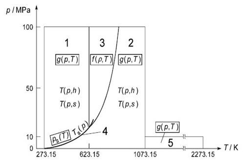
Region 5 has not been implemented in Ansys CFX because it represents a thermodynamic space at very high temperatures (1073.15 - 2273.15 K) and reasonably low pressures (0-10 MPa) that can be adequately described using other property databases already in Ansys CFX (that is, Ideal Gas EOS with NASA specific heat and enthalpy). Furthermore, because this region is not defined for pressures up to 100 MPa, as is the case for regions 1, 2 and 3, problems arise in filling out the pressure-temperature space in the tables when temperatures exceed 1073.15 K and pressures exceed 10 MPa. The database implemented in CFX therefore covers temperatures ranging from 273.15 to 1073.15 K and pressures ranging from 611 Pa to 100 MPa.

The reference state for the IAPWS library is the triple point of water. Internal energy, entropy and enthalpy are all set to zero at this point.

T_ref = 273.16 K, P_ref = 611.657 Pa, u_liquid = 0 J/kg, s_liquid = 0 J/kg/K, h_liquid = 0 J/kg

In Ansys CFX, the analytical equation of state is used to transfer properties into tabular form, which can be evaluated efficiently in a CFD calculation. These IAPWS tables are defined in terms of pressure and temperature, which are then inverted to evaluate states in terms of other property combinations (such as pressure/enthalpy or entropy/enthalpy). When developing the IAPWS database for Ansys CFX, therefore, properties must be evaluated as functions of pressure and temperature. For the most part, this involves a straightforward implementation of the equations described in the IAPWS theory [125]. Region 4 involves saturation data that uses only pressure or temperature information.

However, some difficulties are encountered when evaluating the properties around Region 3 (near the critical point), where the EOS is defined explicitly in terms of density and temperature. In this region, the density must be evaluated using Newton-Raphson iteration. This algorithm is further complicated in that the EOS is applicable on both the subcooled liquid and superheated vapor side leading up to critical conditions. Therefore, depending on the pressure-temperature state, one may be evaluating a subcooled liquid or a superheated vapor with the same EOS. To apply the Newton-Raphson scheme in a reliable way, one must detect on which side of the saturation dome the pressure-temperature state applies, and apply an appropriate initial guess. Such an iteration scheme, including logic for an initial guess, has been implemented in Ansys CFX so that table generation around the critical region is possible.

The IAPWS library also extends to metastable states, so that this equation of state is available for non-equilibrium phase change models such as the Droplet Condensation Model. The EOS for regions 1 and 3 in Figure 1.1: Regions and Equations of IAPWS-IF97 are stated to have reasonable accuracy for metastable states close to the saturation line d liquid states [125]. However, the term "reasonable" is not quantified, and therefore the degree to which the extrapolation of the EOS can be applied is unknown.

In region 2, an additional set of equations have been developed for supercooled vapor conditions under 10 MPa. These equations have been tuned to match the saturation data. Above 10 MPa, the EOS for the superheated region can safely be extrapolated into supercooled conditions, but it does not match smoothly with the specialized supercooled equations below 10 MPa.

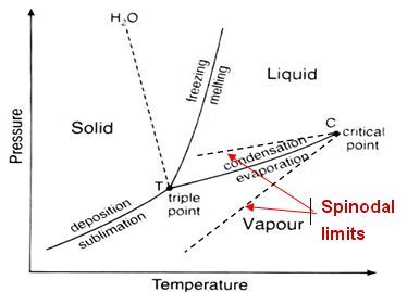
In order to make the IAPWS database as robust as possible, numerical testing has been done to determine approximate metastable vapor/liquid spinodal lines. Figure 1.2: Spinodal Limits Built into Tables is given to demonstrate these spinodal lines that are essentially boundaries up to which metastable conditions can exist. These would be defined similar to saturation curves as functions of either temperature or pressure. The IAPWS database tables are always generated up to these limits regardless of what flow models are specified (equilibrium or non-equilibrium) and therefore allow non-equilibrium phase change models to be applied.

Figure 1.2: Spinodal Limits Built into Tables

The acentric factor must be supplied when running the real gas models and is tabulated for many common fluids in Poling et al. [84]. If you do not know the acentric factor, or it is not printed in a common reference, it can be estimated using knowledge of the critical point and the vapor pressure curve with this formula:

(1–126)

where the vapor pressure, , is calculated at . In addition to the critical point pressure, this formula requires knowledge of the vapor pressure as a function of temperature.