The Time Transformation method handles the problem of unequal pitch described above by transforming the time coordinates of the rotor and stator in the circumferential direction in order to make the models fully periodic in "transformed" time. Let the , , and coordinate axis represent the radial, tangential (pitchwise) and axial directions of the problem described in Figure 4.3: Phase Shifted Periodic Boundary Conditions.

Mathematically, the condition of enforcing the flow spatial periodic boundary conditions on both rotor and stator passages, respectively, is given by:

(4–1)

(4–2)

Alternatively, we can apply the following set of space-time transformations [217] to the problem above as:

(4–3)

(4–4)

(4–5)

(4–6)

where .

The transformed set of equations now has regular spatial periodic boundary conditions as:

(4–7)

(4–8)

And the periodicity is maintained at any instant in time in the computational domain.

There are two important implications of working with the transformed system above instead of the conventional system:

One way of understanding the difference in time step size stated in the second point is:

a) Each passage experiences a different period; that is, the stator period is:

(4–9)

whereas the rotor period is:

(4–10)

b) The period in each passage must be discretized using an identical number of timesteps . We can therefore write the rotor and stator periods as:

(4–11)

(4–12)

where and represent the time step size for the rotor and stator, respectively.

c) Combining the two definitions of rotor and stator periods in a) and b) we have the time step sizes in the rotor and stator related by their pitch ratio as:

(4–13)

The simulation time step size set for the run is used in the stator passage(s) and Ansys CFX computes the respective rotor passage time step size based on the rotor-stator interface pitch ratio as described above.

When the solution is transformed back to physical time, the elapsed simulation time is considered the stator simulation time.

The flow interaction across the rotor-stator interfaces is handled by the pitch scaling machinery already present in the Profile Transformation method. However, while the Profile Transformation method results in a 1:1 pitch ratio with incorrect frequency due to profile contraction or expansion, the Time Transformation method has the correct frequency, as the time has been scaled proportionally.

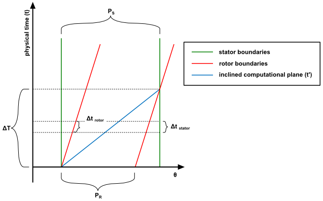
Another way of seeing the difference in time step sizes is to look at the time vs. pitchwise direction plot for both stator and rotor domains. In Figure 4.4: Rotor and stator periodic boundaries in space-time the rotor domain periodic boundaries are plotted with reference to the stator domain. One can notice that, even though the rotor pitch is smaller than the stator pitch in physical space, their boundaries match in the inclined computational space after time . Furthermore, if we look at the time step size of stator and rotor, we see that they are different and related by the rotor-stator pitch ratio.

Figure 4.4: Rotor and stator periodic boundaries in space-time

For modeling information, see Time Transformation in the CFX-Solver Modeling Guide.