


The main advantage of the Time Transformation pitch-change method is that
conventional periodicity
boundary conditions can be applied directly, resulting in relatively fast
convergence.
The Time Transformation method:
Is valid only for compressible flows
Is valid only when the pitch ratio between the modeled components does not deviate much from unity
Requires that the pitch ratio fall within a certain range, as described by the inequality:
where
 is the Mach
number associated with the rotor rotational speed (or signal speed in the case
of an inlet disturbance problem),
is the Mach
number associated with the rotor rotational speed (or signal speed in the case
of an inlet disturbance problem),  is the Mach number associated with the circumferential
velocity, and the ratio of
is the Mach number associated with the circumferential
velocity, and the ratio of  to
to  is the pitch ratio between the stationary component and the
rotating component.
is the pitch ratio between the stationary component and the
rotating component.These limits are not strict, but approaching them can cause solution instability. The CFX-Solver calculates these limits at the start of a simulation and reports them in the CFX-Solver Output file at the beginning of a run.

For most compressible turbomachinery applications (for example, gas compressors and
turbines),  is in the range of 0.3 -
0.6, enabling pitch ratios in the range of 0.6 - 1.5 (Giles [217]). If necessary, you can make the pitch ratio fall within
the permissible range by strategically choosing the number of passages per component for
each of the components.
is in the range of 0.3 -
0.6, enabling pitch ratios in the range of 0.6 - 1.5 (Giles [217]). If necessary, you can make the pitch ratio fall within
the permissible range by strategically choosing the number of passages per component for
each of the components.
Note: See Time Transformation in the CFX-Solver Theory Guide for more theoretical information about the Time Transformation method.
The basic procedure for setting up a Transient Blade Row model is outlined in Setting up a Transient Blade Row Model. For simulations involving the Time Transformation model:
Ensure that the pitch ratio between adjacent components is within the proper range by appropriately adjusting the number of blades in each component. The proper range is described in Time Transformation.
Those transient rotor stator interfaces not referenced by a disturbance will be treated with the Profile Transformation method.
You can model only a single stage. As a result, there must be exactly one domain interface between two time transformed domains.
Based on the case you are working on, for a given domain, add one disturbance to the list of disturbances.
Ensure that the relative speed associated with the disturbance is not zero.
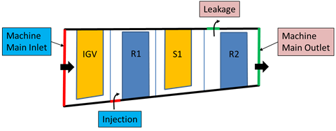
Note: When multiple Time Transformation instances are used, the solver will attempt to compute the streamwise scale equation(*). In cases where the machine contains more than one inlet or outlet (for example, due to the presence of injection holes or cooling grooves) you must manually specify the main inlet and/or main outlet of the machine; that is done by entering the following lines of CCL:
TRANSIENT BLADE ROW MODELS:
   Inflow Boundary = <main inlet name>
   Outflow Boundary = <main outlet name>
   Option = Time Transformation
   .
   .
   .
  END
Failure to specify the main inlet and/or outlet will result in the solver issuing the following message:
Multiple Inlets and/or Openings were detected for this multi-disturbance Time Transformation
  simulation. Please specify one inlet as streamwise scale specified boundary condition region.
(*) The streamwise scale equation is used to compute the streamwise location of the machine components.