


The wall-function approach in Ansys CFX is an extension of the
method of Launder and Spalding [13]. In the log-law region, the near
wall tangential velocity is related to the wall-shear-stress,  , by means of a logarithmic relation.
In the wall-function approach, the viscosity affected sublayer region is bridged by employing empirical formulas to provide near-wall boundary conditions for the mean flow and turbulence transport equations. These formulas connect the wall conditions (for example, the wall-shear-stress) to the dependent variables at the near-wall mesh node, which is presumed to lie in the fully-turbulent region of the boundary layer.
The logarithmic relation for the near wall velocity is given by:
 | (2–219) |
where:
 | (2–220) |
 | (2–221) |
u
+ is the
near wall velocity,  is
the friction velocity, U
t is the known velocity tangent to the wall at a distance of
is
the friction velocity, U
t is the known velocity tangent to the wall at a distance of  from the wall, y
+ is the dimensionless distance from the wall,
from the wall, y
+ is the dimensionless distance from the wall,  is the wall shear stress,
  is the von
Karman constant and C is a log-layer constant
depending on wall roughness (natural logarithms are used).
is the von
Karman constant and C is a log-layer constant
depending on wall roughness (natural logarithms are used).
A definition of  in the different
wall formulations is available in Solver Yplus and Yplus.
in the different
wall formulations is available in Solver Yplus and Yplus.
Equation 2–219 has the problem
that it becomes singular at separation points where the near wall
velocity, U
t, approaches
zero. In the logarithmic region, an alternative velocity scale, u* can be used instead of  :
:
 | (2–222) |
This scale has the useful property that it does not go to zero
if U
t goes to zero. Based
on this definition, the following explicit equation for  can be obtained:
 | (2–223) |
The absolute value of the wall shear stress  , is then obtained from:
 | (2–224) |
where:
 | (2–225) |
and u * is as defined earlier.
One of the major drawbacks of the wall-function approach is that the predictions depend on the location of the point nearest to the wall and are sensitive to the near-wall meshing; refining the mesh does not necessarily give a unique solution of increasing accuracy (Grotjans and Menter [10]). The problem of inconsistencies in the wall-function, in the case of fine meshes, can be overcome with the use of the Scalable Wall Function formulation developed by Ansys CFX. It can be applied on arbitrarily fine meshes and allows you to perform a consistent mesh refinement independent of the Reynolds number of the application.
The basic idea behind the scalable wall-function approach is
to limit the y
* value used in the logarithmic formulation by a lower value of  where 11.06 is the value
of y
* at the intersection
between the logarithmic and the linear near wall profile. The computed
where 11.06 is the value
of y
* at the intersection
between the logarithmic and the linear near wall profile. The computed  is therefore not allowed to fall below this limit.
Therefore, all mesh points are outside the viscous sublayer and all
fine mesh inconsistencies are avoided.
is therefore not allowed to fall below this limit.
Therefore, all mesh points are outside the viscous sublayer and all
fine mesh inconsistencies are avoided.
The boundary condition for the dissipation rate,  , is then given by the
following relation, which is valid in the logarithmic region:
, is then given by the
following relation, which is valid in the logarithmic region:
 | (2–226) |
It is important to note the following points:
To fully resolve the boundary layer, you should put at least 10 nodes into the boundary layer.
Do not use Standard Wall Functions unless required for backwards compatibility.
The upper limit for y + is a function of the device Reynolds number. For example, a large ship may have a Reynolds number of 109 and y + can safely go to values much greater than 1000. For lower Reynolds numbers (for example, a small pump), the entire boundary layer might only extend to around y + = 300. In this case, a fine near wall spacing is required to ensure a sufficient number of nodes in the boundary layer.
If the results deviate greatly from these ranges, the mesh at the designated Wall boundaries will require modification, unless wall shear stress and heat transfer are not important in the simulation.
In most turbulent flows the turbulence kinetic energy is not
completely zero and the definition for  given in Equation 2–222 will give
proper results for most cases. In flows with low free stream turbulence
intensity, however, the turbulence kinetic energy can be very small
and lead to vanishing
given in Equation 2–222 will give
proper results for most cases. In flows with low free stream turbulence
intensity, however, the turbulence kinetic energy can be very small
and lead to vanishing  and therefore also to vanishing wall shear stress,
If this situation happens, a lower limiter can be applied to
and therefore also to vanishing wall shear stress,
If this situation happens, a lower limiter can be applied to  by setting the expert parameter
 ‘ustar limiter = t’.  will then be calculated using the following
relation:
will then be calculated using the following
relation:
 | (2–227) |
The coefficient used in this relation can be changed by setting
the expert parameter ‘ustar limiter coef ‘. The default value of this parameter is 0.01.
In the solver output, there are two arrays for the near wall  spacing. The definition for the Yplus variable that
appears in the post processor is given by the standard definition
of
spacing. The definition for the Yplus variable that
appears in the post processor is given by the standard definition
of  generally
used in CFD:
generally
used in CFD:
 | (2–228) |
where  is the distance
between the first and second mesh points off the wall.
is the distance
between the first and second mesh points off the wall.
In addition, a second variable, Solver Yplus, is available and
contains the  used in the
logarithmic profile by the solver. It depends on the type of wall
treatment used, which can be one of three different treatments in Ansys CFX.
They are based on different distance definitions and velocity scales.
This has partly historic reasons, but is mainly motivated by the desire
to achieve an optimum performance in terms of accuracy and robustness:
used in the
logarithmic profile by the solver. It depends on the type of wall
treatment used, which can be one of three different treatments in Ansys CFX.
They are based on different distance definitions and velocity scales.
This has partly historic reasons, but is mainly motivated by the desire
to achieve an optimum performance in terms of accuracy and robustness:
Standard wall function (based on
 )
)Scalable wall function (based on
 )
)Automatic wall treatment (based on
 )
)
The scalable wall function y + is defined as:
 | (2–229) |
and is therefore based on 1/4 of the near wall mesh spacing.
Note that both the scalable wall function and the automatic wall treatment can be run on arbitrarily fine meshes.
While the wall-functions presented above enable a consistent
mesh refinement, they are based on physical assumptions that are problematic,
especially in flows at lower Reynolds numbers (Re<10
5), as the sublayer portion of the boundary
layer is neglected in the mass and momentum balance. For flows at
low Reynolds numbers, this can cause an error in the displacement
thickness of up to 25%. It is therefore desirable to offer
a formulation which will automatically switch from wall-functions
to a low-Re near wall formulation as the mesh
is refined. The  model of Wilcox has the advantage that an analytical
expression is known for
model of Wilcox has the advantage that an analytical
expression is known for  in the viscous sublayer, which
can be exploited to achieve this goal. The main idea behind the present
formulation is to blend the wall value for
in the viscous sublayer, which
can be exploited to achieve this goal. The main idea behind the present
formulation is to blend the wall value for  between the
logarithmic and the near wall formulation.
between the
logarithmic and the near wall formulation.
The automatic wall treatment allows a consistent y + insensitive mesh refinement from coarse meshes, which do not resolve the viscous sublayer, to fine meshes placing mesh points inside the viscous sublayer. Note that for highly accurate simulations, like heat transfer predictions, a fine mesh with y + around 1 is recommended.
The flux for the k-equation is artificially kept to be zero and the flux in the momentum equation is computed from the velocity profile. The equations are as follows:
Flux for the momentum equation, F U:
 | (2–230) |
with:
 | (2–231) |
 | (2–232) |
where

and

Flux for the k-equation:
 | (2–233) |
In the  -equation, an algebraic expression
is specified instead of an added flux. It is a blend between the analytical
expression for
-equation, an algebraic expression
is specified instead of an added flux. It is a blend between the analytical
expression for  in the logarithmic region:
 | (2–234) |
and the corresponding expression in the sublayer:
 | (2–235) |
with  being the distance
between the first and the second mesh point. In order to achieve a
smooth blending and to avoid cyclic convergence behavior, the following
formulation is selected:
being the distance
between the first and the second mesh point. In order to achieve a
smooth blending and to avoid cyclic convergence behavior, the following
formulation is selected:
 | (2–236) |
While in the wall-function formulation, the first point is treated
as being outside the edge of the viscous sublayer; in the low-Re mode, the location of the first mesh point is virtually
moved down through the viscous sublayer as the mesh is refined. Note
that the physical location of the first mesh point is always at the
wall (y = 0). However, the first
mesh point is treated as if it were  y away from the wall. The error in the wall-function formulation results
from this virtual shift, which amounts to a reduction in displacement
thickness. Also, at very low Reynolds numbers this shift becomes visible
when the solution is compared with a laminar calculation, because
the shift is not needed in the laminar near wall treatment. This error
is always present in the wall-function model. The shift is based on
the distance between the first and the second mesh point
y away from the wall. The error in the wall-function formulation results
from this virtual shift, which amounts to a reduction in displacement
thickness. Also, at very low Reynolds numbers this shift becomes visible
when the solution is compared with a laminar calculation, because
the shift is not needed in the laminar near wall treatment. This error
is always present in the wall-function model. The shift is based on
the distance between the first and the second mesh point  y = y
2
- y
1 with y being the wall normal distance.
y = y
2
- y
1 with y being the wall normal distance.
The near wall treatment that was discussed above (Scalable Wall Functions, Automatic Wall Treatment) is appropriate when walls can be considered as hydraulically smooth. Surface roughness can have a significant effect on flows of engineering interest. Surface roughness typically leads to an increase in turbulence production near the wall. This in turn can result in significant increases in the wall shear stress and the wall heat transfer coefficients. For the accurate prediction of near wall flows, particularly with heat transfer, the proper modeling of surface roughness effects is essential for a good agreement with experimental data.
Wall roughness increases the wall shear stress and breaks up the viscous sublayer in turbulent flows. The figure below (Figure 2.6: Downward Shift of the Logarithmic Velocity Profile) shows the downward shift in the logarithmic velocity profile:
 | (2–237) |
where B=5.2. The shift  is a function of
the dimensionless roughness height,
is a function of
the dimensionless roughness height,  ,
defined as
,
defined as  .
.
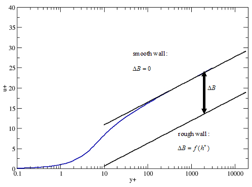
For sand-grain roughness, the downward shift can be expressed as:
 | (2–238) |
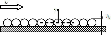
It has been shown that a technical roughness, which has peaks
and valleys of different shape and size, can be described by an equivalent
sand-grain roughness ([113], [77]). The corresponding
picture is a wall with a layer of closely packed spheres, which have
an average roughness height  (see Figure 2.7: Equivalent Sand-Grain Roughness):
Guidance to determine the appropriate equivalent sand-grain roughness height can be obtained from White [14], Schlichting [77] and Coleman et al. [193].
Depending on the dimensionless sand-grain roughness  , three roughness regimes can be distinguished:
hydraulically smooth wall :

transitional-roughness regime:

fully rough flow:

The viscous sublayer is fully established near hydraulically smooth walls. In the transitional roughness regime the roughness elements are slightly thicker than the viscous sublayer and start to disturb it, so that in fully rough flows the sublayer is destroyed and viscous effects become negligible.
From the picture of the sand-grain roughness (note that Figure 2.7: Equivalent Sand-Grain Roughness shows a two-dimensional cut of a three-dimensional arrangement), it can be assumed that the roughness has a blockage effect, which is about 50% of its height. The idea is to place the wall physically at 50% height of the roughness elements:
 | (2–239) |
This gives about the correct displacement caused by the surface roughness.
The Scalable Wall Function approach neglects the viscous sublayer
and limits the value used in the logarithmic formulation by a lower
value of  (Equation 2–229). This limiter must be combined with the formulation Equation 2–239 for the rough wall
treatment and reads:
(Equation 2–229). This limiter must be combined with the formulation Equation 2–239 for the rough wall
treatment and reads:
 | (2–240) |
The automatic wall treatment works well for smooth walls and
has been extended for rough walls. However, any calibration of the
model coefficients has to be performed for both  and
and  and is therefore more complex than for smooth walls. As outlined
above, the viscous sublayer gets more and more disturbed with increasing
values of
and is therefore more complex than for smooth walls. As outlined
above, the viscous sublayer gets more and more disturbed with increasing
values of  until it is destroyed
in fully rough flows. Therefore, a blending between the viscous sublayer
and the logarithmic region is not physical for large values of
until it is destroyed
in fully rough flows. Therefore, a blending between the viscous sublayer
and the logarithmic region is not physical for large values of  . This fact supports the idea of placing the wall physically at 50%
height of the roughness elements. Due to this shift, the viscous sublayer
formulation has only an influence for small values of
. This fact supports the idea of placing the wall physically at 50%
height of the roughness elements. Due to this shift, the viscous sublayer
formulation has only an influence for small values of  in the automatic near wall treatment for rough walls. The blending
between the viscous sublayer formulation and the wall function is
described in detail in the report Lechner and Menter [194].
in the automatic near wall treatment for rough walls. The blending
between the viscous sublayer formulation and the wall function is
described in detail in the report Lechner and Menter [194].
Because the automatic wall treatment works together with the transition model, it is the default rough wall treatment. This default Automatic setting for the Wall Function option can be set on the Fluid Models tab of the Domain details view in CFX-Pre. The CFX-Solver checks internally if a roughness height has been specified for a wall and then uses the proper wall treatment: when a roughness height exists, then the automatic rough wall treatment is used, otherwise the automatic smooth wall treatment.
If the two-equation transition model (Gamma Theta Model) is used together with rough walls, then the option Roughness Correlation must be turned on in CFX-Pre on the Fluid Models tab in order to take the roughness effects into account in the transition model. Setting the sand-grain roughness height at a wall alone is not sufficient. The roughness correlation requires the geometric roughness height as input parameter because it turned out that for the transition process from laminar to turbulent flow, the geometric roughness height is more important than the equivalent sand-grain roughness height. The correlation is defined as
 | (2–241) |
where the function  depends on the geometric roughness
height
depends on the geometric roughness
height  . This function is proprietary
and therefore not given in this documentation.
. This function is proprietary
and therefore not given in this documentation.  is then used in the correlations for
  and
and  (Equation 2–150 and Equation 2–151) instead of
  , which represents the transition momentum
thickness Reynolds number (for details, see Ansys CFX Laminar-Turbulent Transition Models). In other words the roughness effect is taken into account by
using a modified transition momentum thickness Reynolds number in
the correlations for
, which represents the transition momentum
thickness Reynolds number (for details, see Ansys CFX Laminar-Turbulent Transition Models). In other words the roughness effect is taken into account by
using a modified transition momentum thickness Reynolds number in
the correlations for  and
and  .
.
Consequently the shift in Equation 2–239 was redefined as the minimum of either the
geometric roughness height  or the sand grain roughness height
  as follows:
 | (2–242) |
The fact that the viscous sublayer is lost very quickly with
increasing  suggests to neglect
the viscous sublayer in the formulation of a near wall treatment for
rough walls and leads to a second rough wall treatment for
suggests to neglect
the viscous sublayer in the formulation of a near wall treatment for
rough walls and leads to a second rough wall treatment for  -based turbulence models.
It should only be used if you know that the influence of the viscous
sublayer can be neglected (
-based turbulence models.
It should only be used if you know that the influence of the viscous
sublayer can be neglected ( > 70) and if the
flow is fully turbulent. It can only be enabled by extracting the
CCL and changing the Wall Function from
> 70) and if the
flow is fully turbulent. It can only be enabled by extracting the
CCL and changing the Wall Function from Automatic to Scalable.
Then scalable wall functions are used both for smooth and rough
walls for the  -based turbulence models. The idea is comparable
to the scalable wall function approach for the
-based turbulence models. The idea is comparable
to the scalable wall function approach for the  model, where the first mesh point is shifted
to the edge of the viscous sublayer and only the relations of the
logarithmic region are used to derive the boundary conditions. In
order to avoid a negative logarithm in the logarithmic law of the
wall, a lower value of 11.06 is defined in the following manner:
model, where the first mesh point is shifted
to the edge of the viscous sublayer and only the relations of the
logarithmic region are used to derive the boundary conditions. In
order to avoid a negative logarithm in the logarithmic law of the
wall, a lower value of 11.06 is defined in the following manner:
 | (2–243) |
where  .
.
It should be noted that this value is smaller than the lower
limit in the scalable wall functions of the  model because for rough walls, the log
layer extends to smaller values of
model because for rough walls, the log
layer extends to smaller values of  .
Because the scalable wall function approach neglects the viscous sublayer,
the diffusion coefficients in the Navier-Stokes and turbulence transport
equations must no longer be computed as the sum of the laminar and
turbulent viscosity. Instead the maximum value of the both is used.
In the momentum equation for example the effective viscosity will
be computed as
.
Because the scalable wall function approach neglects the viscous sublayer,
the diffusion coefficients in the Navier-Stokes and turbulence transport
equations must no longer be computed as the sum of the laminar and
turbulent viscosity. Instead the maximum value of the both is used.
In the momentum equation for example the effective viscosity will
be computed as
 | (2–244) |
Note that the logarithmic layer formulation is only correct if the molecular viscosity is not included in the equations. This is ensured by the above formulation.
An additional model, High Roughness (Icing), is available for the SST
model. This model is primarily designed and tested for icing applications. However
this model is generally useful for all roughness applications and has shown
improved results relative to the standard rough wall model, for cases where the roughness
height is not small relative to the boundary layer thickness. Note that, for the standard
model, the roughness height must be less than the log-layer thickness,
the latter typically being around 20% of the boundary layer thickness.
Note: The High Roughness (Icing) model requires a fine near-wall grid
spacing of the order of  .
.
The model is based on the concept of non-zero eddy viscosity on the wall. It is estimated by
modeling the wall values of k and  in accordance with the Colebrook correlation by Aupoix [230]. Because the roughness effect is strong, the turbulent
viscosity should be large compared to the laminar viscosity at the wall. Specifically,
Aupoix proposed the following formulations to compute the non-dimensional k and
in accordance with the Colebrook correlation by Aupoix [230]. Because the roughness effect is strong, the turbulent
viscosity should be large compared to the laminar viscosity at the wall. Specifically,
Aupoix proposed the following formulations to compute the non-dimensional k and
 on a wall
  ,
,  [230]:
 | (2–245) |
 | (2–246) |
where  is a standard constant in the SST model, and
  and
and  are defined as:
 | (2–247) |
 | (2–248) |
Therefore, all the wall values of k and  are known:
 | (2–249) |
 | (2–250) |
No wall shift (like Equation 2–239) is performed for this model.
Heat flux at the wall can be modeled using the scalable wall function approach or the automatic wall treatment. Using similar assumptions as those above, the non-dimensional near-wall temperature profile follows a universal profile through the viscous sublayer and the logarithmic region. The non-dimensional temperature, T +, is defined as:
 | (2–251) |
where T w is the temperature at the wall, T f the near-wall fluid temperature, c p the fluid heat capacity and q w the heat flux at the wall. The above equation can be rearranged to get a simple form for the wall heat flux model:
 | (2–252) |
Turbulent fluid flow and heat transfer problems without conjugate heat transfer objects require the specification of the wall heat flux, q w, or the wall temperature, T w. The energy balance for each boundary control volume is completed by multiplying the wall heat flux by the surface area and adding to the corresponding boundary control volume energy equation. If the wall temperature is specified, the wall heat flux is computed from the equation above, multiplied by the surface area and added to the boundary energy control volume equation.
For scalable wall functions, the non-dimensional temperature profile follows the log-law relationship:
 | (2–253) |
where  is defined
in Equation 2–229 and
is defined
in Equation 2–229 and  is
computed from Equation 2–255.
is
computed from Equation 2–255.
For the automatic wall function, the thermal boundary layer is modeled using the thermal law-of-the-wall function of B.A. Kader [15]. Then, the non-dimensional temperature distribution is modeled by blending the viscous sublayer and the logarithmic law of the wall. This can be modeled as:
 | (2–254) |
where:
 | (2–255) |
 | (2–256) |
Pr is the fluid Prandtl number, given by:
 | (2–257) |
where  is the fluid thermal conductivity.
It can be shown for a flat plate with heat transfer that the
wall heat flux is under-predicted if the logarithmic law of the wall
for the temperature is used in the form which has been derived for
smooth walls. Based on the idea that for  the velocity and temperature logarithmic laws of the wall are the
same for smooth walls, the logarithmic law of the wall for the temperature
has been extended in a similar way as the one for the velocity to
account for the wall roughness effect. But instead of the roughness
height Reynolds number
the velocity and temperature logarithmic laws of the wall are the
same for smooth walls, the logarithmic law of the wall for the temperature
has been extended in a similar way as the one for the velocity to
account for the wall roughness effect. But instead of the roughness
height Reynolds number  , the formulation is
based on
, the formulation is
based on  due to the influence of the Prandtl
number that has already been accounted for in the smooth wall formulation.
A calibration constant has been introduced because the Kader logarithmic
law of the wall is not strictly identical with the velocity log law
for
due to the influence of the Prandtl
number that has already been accounted for in the smooth wall formulation.
A calibration constant has been introduced because the Kader logarithmic
law of the wall is not strictly identical with the velocity log law
for  . It should also be noted
that roughness elements introduce pressure-drag on the sides of the
elements, which is not present in the thermal formulation. The coefficient
by which the thermal layer has to be shifted is therefore expected
to be smaller than one. The shift has been introduced in the rough
wall treatment of both
. It should also be noted
that roughness elements introduce pressure-drag on the sides of the
elements, which is not present in the thermal formulation. The coefficient
by which the thermal layer has to be shifted is therefore expected
to be smaller than one. The shift has been introduced in the rough
wall treatment of both  and
and  -based turbulence
models. The modification of the logarithmic law of the wall for the
temperature reads:
-based turbulence
models. The modification of the logarithmic law of the wall for the
temperature reads:
 | (2–258) |
where

The coefficient  has been calibrated using the experimental data
of Pimenta et al. [195] for a flat plate with
heat transfer. The experiment was performed with air as fluid and
it has been shown, that a value of 0.2 is a good choice in this case
(Lechner and Menter [194]). Therefore the default value
of
has been calibrated using the experimental data
of Pimenta et al. [195] for a flat plate with
heat transfer. The experiment was performed with air as fluid and
it has been shown, that a value of 0.2 is a good choice in this case
(Lechner and Menter [194]). Therefore the default value
of  is 0.2. This coefficient is called Energy
Calibration Coefficient and can be changed in the CCL if
necessary in the following way:
is 0.2. This coefficient is called Energy
Calibration Coefficient and can be changed in the CCL if
necessary in the following way:
     FLUID MODELS:
       ...
       TURBULENCE MODEL:
         Option = SST
       END
       TURBULENT WALL FUNCTIONS:
         Option = Automatic
         Energy Calibration Coefficient = 0.2
       END
       ...
     END
If the wall function approach for  -based turbulence
models is used, two additional points have to be considered.
-based turbulence
models is used, two additional points have to be considered.
Similar to Equation 2–243 a lower limit for
 ,
which appears in the equation of
,
which appears in the equation of  ,
has been introduced. A value of 11.06 was chosen as lower limit:
,
has been introduced. A value of 11.06 was chosen as lower limit:
(2–259)
Because the scalable wall function approach neglects the viscous sublayer, the following relation is automatically used to compute the effective conductivity
 :
:
(2–260)
With increasing Mach number (Ma > 3), the accuracy of the wall-functions approach degrades, which can result in substantial errors in predicted shear stress, wall heat transfer and wall temperature for supersonic flows.
It has been found that the incompressible law-of-the-wall is also applicable to compressible flows if the velocity profile is transformed using a so-called "Van Driest transformation" [16]. The logarithmic velocity profile is given by:
 | (2–261) |
where  ,
,  ,
,  = 0.41 and C = 5.2. The subscript w refers to wall conditions, and the subscript "comp"
refers to a velocity defined by the following equation (transformation):
= 0.41 and C = 5.2. The subscript w refers to wall conditions, and the subscript "comp"
refers to a velocity defined by the following equation (transformation):
 | (2–262) |
Near a solid wall, the integrated near-wall momentum equation reduces to:
 | (2–263) |
while the energy equation reduces to:
 | (2–264) |
Expressions for shear stress and heat flux applicable to the boundary layer region are:
 | (2–265) |
and
 | (2–266) |
If Equation 2–263, Equation 2–265 and Equation 2–266 are substituted into Equation 2–264 and integrated, the resulting equation is:
 | (2–267) |
which provides a relationship between the temperature and velocity profiles. Using the perfect gas law, and the fact that the pressure is constant across a boundary layer, Equation 2–267 replaces the density ratio found in Equation 2–262. Performing the integration yields the following equation for the "compressible" velocity:
 | (2–268) |
where:
 | (2–269) |
 | (2–270) |
 | (2–271) |
The above derivation provides most of the equations necessary for the implementation of wall-functions that are applicable to compressible flows. These wall-functions are primarily implemented in two locations in Ansys CFX: hydrodynamics and energy. First, consider the implementation in the hydrodynamics section. The equation for the wall-shear-stress is obtained after a slight rearrangement of Equation 2–261:
 | (2–272) |
This is similar to the low speed wall-function, except that U comp now replaces U. The Van Driest transformation given by Equation 2–268, must now be performed on the near wall velocity. In the implementation, Equation 2–268 is re-written in the following form:
 | (2–273) |
where:
 | (2–274) |
This completes the wall-function modifications for the hydrodynamics.
The relationship between wall heat transfer, near wall velocity
and near wall temperature is given by Equation 2–267 (and also in rearranged form after Equation 2–273: the equation for T
w
/ T). A dimensionless variable,  ,
can be defined as:
,
can be defined as:
 | (2–275) |
and hence:
 | (2–276) |
From Equation 2–276 it is clear
that knowing  ,
the near wall velocity, the near wall temperature and the wall heat
transfer, the wall temperature can be calculated (if instead the wall
temperature is known, then the wall heat transfer is calculated).
Before proceeding, it is instructive to consider the equation that
is used in Ansys CFX for low Mach number heat transfer. The equation
is subsequently modified for use at higher Mach numbers. This unmodified
equation is given by:
,
the near wall velocity, the near wall temperature and the wall heat
transfer, the wall temperature can be calculated (if instead the wall
temperature is known, then the wall heat transfer is calculated).
Before proceeding, it is instructive to consider the equation that
is used in Ansys CFX for low Mach number heat transfer. The equation
is subsequently modified for use at higher Mach numbers. This unmodified
equation is given by:
 | (2–277) |
where:
 | (2–278) |
 | (2–279) |
 | (2–280) |
 | (2–281) |
It can be seen that this equation blends between the linear and logarithmic near wall regions, and hence is more general than just using the logarithmic profile that is implied by Equation 2–275. Equation 2–277 has been extended for use in the compressible flow regime by interpreting the linear and logarithmic velocity profiles given above as "compressible" or Van Driest transformed velocities:
 | (2–282) |
 | (2–283) |
This change is consistent with Equation 2–261. The "untransformed" velocities required by Equation 2–277 can be obtained by applying the inverse Van Driest velocity transformation to these "compressible" velocities. The inverse transformation is given by:
 | (2–284) |
where:
 | (2–285) |
 | (2–286) |
and A and B are defined following Equation 2–268 above. The reverse transformed velocities obtained
from Equation 2–284 are substituted
into Equation 2–277 to obtain the
value of  .
Either the wall heat transfer or the wall temperature can then be
obtained from Equation 2–276.
.
Either the wall heat transfer or the wall temperature can then be
obtained from Equation 2–276.
The Van Driest transformation described above is used when High Speed (compressible) Wall Heat Transfer Model is selected in CFX-Pre, in the Domain details view:
On the Fluid Models tab, under Turbulence, or
For a multiphase case with a fluid-specific turbulence model, on the Fluid Specific Models tab.
This option is available only in combination with the Total Energy heat-transfer model.