


The use cases targeted with these multi-blade row models include:
The transient rotor stator (TRS) single stage case is supported by the following pitch-change methods: Profile Transformation, Time Transformation, and Fourier Transformation. Each method has different requirements:
Profile Transformation
For each component, you can model one (or an arbitrary number of) passage(s).
Harmonic Analysis is available; for details, see Profile Transformation and Fourier Transformation using Harmonic Analysis.
Time Transformation
You must select the transient rotor stator interface to which the transformation applies.
No additional parameters are needed if the 'Automatic' selection of domains is applied for either side of the interface.
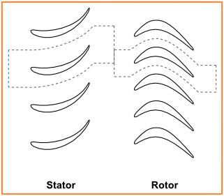
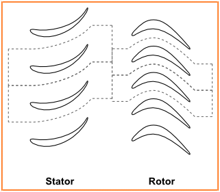
Fourier Transformation
For each component, you must model two instances of the domain, or group of domains (see Fourier Transformation: Workflow Requirements).
You must select the transient rotor stator interface to which this transformation applies.
You must specify, for each domain connected to the rotor-stator interface: (a) which interface is the sampling interface and (b) which interface is the phase-shifted periodic interface (to be used for the application of phase-corrections).
Harmonic Analysis is available; for details, see Profile Transformation and Fourier Transformation using Harmonic Analysis.

A single-stage rotor-stator simulation can be performed using the Profile Transformation or Fourier Transformation pitch-change method. Compared to a time-marching simulation, a significant reduction in computational time can be achieved by performing the simulation using the Harmonic Analysis (HA) solution method, which avoids the need for solving in time over many disturbance periods in order to reach a steady-periodic state. For details, see Harmonic Analysis in the CFX-Solver Theory Guide.
A single-stage rotor-stator simulation that uses the HA methodology is set up like a single-stage rotor-stator simulation that uses the time-marching method, except:
In the Transient Blade Row Models details view, on the Basic Settings tab, you must set Transient Method > Option to
Harmonic Balanceand Transient Method > Number of Modes to an appropriate value (usually 3 or larger).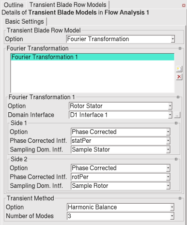
For a Profile Transformation with HA, you must also specify the time period, either by providing a value or by specifying the passing period of a rotating domain.
In the Solver Control details view, on the Basic Settings tab, ensure that Transient Scheme > Option is set to
Harmonic Balance, specify the maximum number of iterations (Max. Iterations), and set the pseudo-time step size (Fluid Timescale Control settings). Typically, the size of the pseudo-time step (Physical Timescale) is equal to the rotor blade passing period divided by the intended number of pseudo-time steps per period.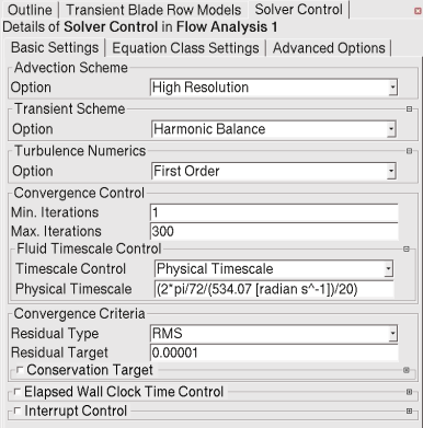
A typical number of pseudo-time steps per period is between 15 and 30. Recall that the lower the number of pseudo-time steps that can be used while maintaining a stable solution, the more efficient the calculation is with respect to the time marching method.
A flow boundary disturbance case involves modeling the effect of an external component (a virtual blade row upstream or downstream of the fluid mesh) via an inlet or outlet boundary condition that varies in time. Such cases are supported by the Time Transformation and Fourier Transformation models.
This type of simulation can be used as a lower-order approximation to a stage simulation. In inlet disturbance simulations the upstream component is modeled by prescribing a profile that is at the inlet and that models the wake of the upstream component.
You can prescribe wake profiles via CEL expressions or via external
*.csv files. CEL-based profiles need not be formulated
to produce rotational motion in time. If a profile does not cover the whole 360°
wheel, then it should consist of a periodic portion that can be replicated to
produce a 360° profile. You may optionally produce a 360° profile in a
*.csv file based on a smaller profile file by using the
Edit Profile Data dialog box in CFX-Pre (see Edit Profile Data in the CFX-Pre User's Guide).
Whether using a CEL expression or a *.csv file, you can
cause the profile data to move (typically rotationally, about the machine axis) by
associating the boundary with a moving coordinate frame. For details, see:
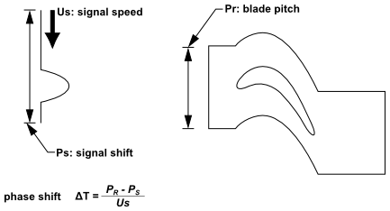
For a rotational-flow disturbance case, the required External Passage
Definition input parameters are aimed at specifying the pitch of the
profile (or signal) at the inlet/outlet. These are needed to help compute the phase
shift ( of Figure 6.5: Inlet Disturbance Case).
These parameters are important to guarantee that the resultant signal has periodic
behavior.
of Figure 6.5: Inlet Disturbance Case).
These parameters are important to guarantee that the resultant signal has periodic
behavior.
As described above, a Flow Boundary Disturbance calculation can be performed on two blade passages using the Fourier-Transformation pitch-change method. The solution is obtained faster than for a full-wheel calculation. A significant further reduction in computational time can be achieved by performing the computation using the Harmonic Analysis (HA) (see Harmonic Analysis in the CFX-Solver Theory Guide) solution method, which avoids the need for solving in time over many disturbance periods in order to reach a steady-periodic state.
A flow boundary disturbance simulation that uses the HA methodology is set up like a flow boundary disturbance simulation that uses the time-marching method, except:
In the Transient Blade Row Models details view, on the Basic Settings tab, you must set Transient Method > Option to
Harmonic Balanceand Transient Method > Number of Modes to an appropriate value.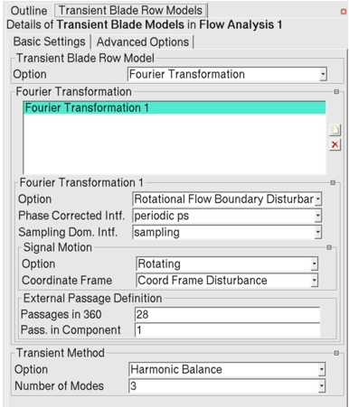
In the Solver Control details view, on the Basic Settings tab, ensure that Transient Scheme > Option is set to
Harmonic Balance, specify the maximum number of iterations (Max. Iterations), and set the pseudo-time step size (Fluid Timescale Control settings). Typically, the size of the pseudo-time step (Physical Timescale) is equal to the disturbance period divided by the intended number of pseudo-time steps per period.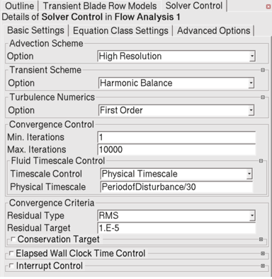
A typical number of pseudo-time steps per period is between 15 and 30. Recall that the lower the number of pseudo-time steps that can be used while maintaining a stable solution, the more efficient the calculation is with respect to the time marching method.
A multi-disturbance gust analysis can be modeled using the Fourier Transformation method. In this analysis, the blade is subjected to two simultaneous disturbances; one on the inlet and the other on the outlet of the blade passage. Typically, the inlet and outlet profiles are initially extracted from a steady-state stage simulation of a 1.5 stage configuration. The profiles are then imposed on the inlet and outlet of the rotor passage in a transient gust simulation. This modeling strategy can be used as an alternative for modeling a 1.5 stage compressor or turbine. It accounts for blade passing frequencies from the upstream and downstream rows on the modeled blades. The use of the Fourier Transformation method also allows for very large pitch variations such as with a fan subjected to inflow distortion.
In general, the procedure to set up a multi-disturbance gust analysis with the Fourier Transformation method closely follows the setup of an inlet disturbance problem with the Fourier Transformation method (see Fourier Transformation Disturbance Settings in the CFX-Pre User's Guide). Note the following important steps:
After setting up the first disturbance, you must add a second disturbance from the same Transient Blade Row Models details view.
Using the Transient Analysis Method:
Specifying the time step in the Transient Blade Row Models details view requires two steps: (1) Specifying a meaningful time period under Transient Method > Time Period. This can be the period of one of the disturbances or the common period between all the disturbances; (2) Specifying Timesteps/Period.
Using the Harmonic Analysis Method:
In the Transient Blade Row Models details view, the number of modes needs to be specified under Transient Method > Number of Modes. This represents the number of harmonics of each of the disturbances that will be used in the simulation. For example, specifying 3 modes for a case that has 2 boundary disturbances will result in 6 modes and will require a total of 13 time planes to solve.
Ensure that all the boundary disturbances are set up correctly. For example, in a two-disturbance case (inlet and outlet) both inlet and outlet boundary conditions must now be specified with a disturbance either through CEL or specified profiles.
For stationary disturbances, ensure that you create and refer to a stationary coordinate frame in the Boundary details view as well as the Transient Blade Row Models details view.
Note:
It is not ideal to use this modeling technique if strong outlet recirculation is present at the boundary.
If the case is not periodic by nature then this modeling method will either artificially make the solution periodic or the solution may fail to converge.
Aerodynamic damping calculations are used in the design of turbines, compressors, and fans to predict failures due to blade flutter and to estimate blade life cycles.
Blade flutter and damping calculations can be performed in Ansys CFX by solving for flow over vibrating blades with prescribed blade displacements. Blade flutter usually occurs at the natural frequency of the blade-disc assembly. This natural frequency can be determined, along with blade displacements (mode shapes), using Ansys Mechanical prior to performing a flow analysis on the blade. In general, the natural disc frequency of a rotor-disc assembly consists of many modes. However, only a limited number of these modes contribute to flutter and only these modes are considered during a blade flutter simulation setup.
For blade flutter calculations, it is important to consider the aerodynamic
effects of adjacent blades. For a rotor-disc assembly consisting of
 blades, there is a finite number of disc nodal
diameters. At nodal diameter
blades, there is a finite number of disc nodal
diameters. At nodal diameter  , all the
blades vibrate in phase with an Interblade Phase Angle (IBPA) of
, all the
blades vibrate in phase with an Interblade Phase Angle (IBPA) of
0. However, for other nodal diameters, each blade will be
out of phase with respect to the others by a finite interblade phase angle value.
The interblade phase angle can be computed from the nodal diameter as:
 | (6–1) |
where
 for an even number of blades and
 for an odd number of blades.
In CFX you can set up a full domain transient model to perform a blade flutter simulation. Alternatively, you can use the Fourier Transformation method to perform a blade flutter analysis using a truncated domain with two passages.
The main objective of a blade flutter analysis is to obtain the aerodynamic damping, or work per vibration cycle. Once a transient periodic solution is achieved, you can use the energy balance method to perform the damping calculation. This calculation yields a measure of the system stability at each nodal diameter and blade vibration frequency. The work per vibration cycle can be computed as:
 | (6–2) |
Where:
 (that is, the period of one vibration cycle)
 is the time at the start of the vibration cycle.
 is the vibration frequency (that is, the
Frequency value specified on the
Boundary Details tab; see Periodic Displacement in the CFX-Solver Modeling Guide)
is the vibration frequency (that is, the
Frequency value specified on the
Boundary Details tab; see Periodic Displacement in the CFX-Solver Modeling Guide) is the fluid pressure
 is
the velocity of the blade due to imposed vibrational
displacements
is
the velocity of the blade due to imposed vibrational
displacements is the surface area (in this case, the surface of the
blade)
is the surface area (in this case, the surface of the
blade) is the surface
normal unit vector.
is the surface
normal unit vector.
Note: Positive values for work indicate that the vibration is damped (for the frequency being studied), whereas negative values indicate that the vibration is undamped.
Aerodynamic damping monitors can be used to monitor aerodynamic damping during a run. The monitor value is calculated according to Equation 6–2 subject to the following modifications and conditions:
The integration limits are set to encompass an integration interval rather than a vibration cycle. The integration interval size is a multiple of the period of one vibration cycle, the multiple being the value specified for the Integration Multiplier setting, described at [Aerodynamic Damping Name]: Integration Multiplier in the CFX-Pre User's Guide. The resulting integral, which represents the work done over the course of one integration interval, is divided by the integration multiplier. For an integration multiplier of one (default), the result is the (unnormalized) aerodynamic damping value. For an integration multiplier greater than one, the result is an average value of (unnormalized) aerodynamic damping (work per vibration cycle) as evaluated over the integration interval (that is, multiple vibration cycles).
The upper time limit on the integral can be at the end of the last complete integration interval or at the current time step, depending on whether the aerodynamic damping option (described at [Aerodynamic Damping Name]: Option in the CFX-Pre User's Guide) is set to
Full Period IntegrationorMoving Integration Interval, respectively.The resulting value (unnormalized aerodynamic damping) is then divided by the specified normalization value, described at [Aerodynamic Damping Name]: Normalization in the CFX-Pre User's Guide, to yield a normalized value of aerodynamic damping for the aerodynamic damping monitor.
Note: After a new run is started, an aerodynamic damping monitor reports a value of zero until the required integration interval has passed.
For each component, you must model two instances of the passage, or group of passages, that is repeatable (see Fourier Transformation: Workflow Requirements).
The vibration of the blades with Interblade Phase Angle (IBPA) results in a traveling wave pattern.
To complete the model, you must specify the following information:
The modal Frequency.
Information about the traveling wave.
This information can be specified using one of the Phase Angle options for a boundary that has the
Periodic Displacementmesh motion option (see Periodic Displacement). For example, with theNodal Diameter (Phase Angle Multiplier)option, you can specify the traveling wave direction:ForwardorBackward.
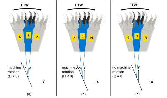
For the traveling wave direction, the direction considered to be forward is (by default):
For a model that has a rotating component: the direction of machine rotation. A Forward Traveling Wave (FTW) is associated with a positive IBPA value. Parts (a) and (b) of Figure 6.7: Direction of Forward Traveling Wave show the forward direction for a rotating component.
For a model that has only stationary components (for example, a model of a stand-alone stator): the direction of increasing sector tag number. Part (c) of Figure 6.7: Direction of Forward Traveling Wave shows the forward direction for a component in a model having no rotating components.
Note: You can change which direction is considered to be forward (corresponding to a positive phase angle). For details,
see the description for expert parameter meshdisp phase angle convention given in Physical Model Parameters.
In CFX, sector tagging is independent of machine rotation. The sector tag number starts at 1 (one) for the original sector and, as shown in Figure 6.7: Direction of Forward Traveling Wave, increases around the wheel in a direction established using the right hand rule and the global coordinate frame.
To compute the magnitude of the nodal diameter, divide the magnitude of the IBPA by the blade
pitch in radians. The magnitude of the IBPA can be defined as
 , where
  is the time shift between adjacent blades. The blade pitch in radians is
  ,
where
,
where  is the number of blades. The
magnitude of the nodal diameter can therefore be computed as
is the number of blades. The
magnitude of the nodal diameter can therefore be computed as  .
.
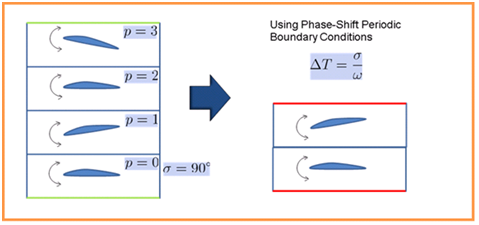
Note: The size of the computational model for the analysis of a blade flutter case that uses standard periodicity boundary conditions, such as the one illustrated in Figure 6.6: Application of Phase-Shifted Boundaries to a Blade Flutter Case, is heavily dependent on the number of passages and the nodal diameter. For most cases, a large sector of the blade row must be modeled. When you account for the phase shift at periodic boundaries by using the Fourier Transformation method, the computational model only needs to include two passages for any nodal diameter.
Note: If splitter blades are involved, then for the purpose of calculating the magnitude of the nodal diameter, the blade pitch should be measured from one main blade to the next.
Note: For cases where the mesh motion on a given boundary straddles stationary interfaces, there is a risk of mesh folding. In order to prevent this problem, the Ansys CFX-Solver automatically blends the mesh motion displacement amplitude down to zero on boundary nodes approaching the stationary interfaces. This strategy, referred to as "Zero Displacement Approximation", is always used because the Fourier Transformation Blade Flutter model requires stationary interfaces. The "Zero Displacement Approximation" might be the cause of solution discrepancies between a Fourier Transformation Blade Flutter model and its equivalent Symmetric Blade Flutter case, for example, when the displacements across stationary interfaces are large compared to displacements elsewhere in the domain.
The fundamental input, which is the modal shape of the structure, must be computed and provided in the Ansys CFX .csv file format (see Profile Data Format in the CFX-Pre User's Guide). This file should contain the coordinates, real modal displacements, and complex modal displacements (only for cyclic symmetry models) at the structural mesh locations. For cyclic symmetry cases (usually involving complex mode shapes), the harmonic index (nodal diameter) should also be provided. A sample .csv mode shape profile is shown below. If the mode shape profile was calculated by Ansys Mechanical then System Coupling tools can be used to prepare the .csv file in the correct format. See Aerodynamic Damping Analysis in the System Coupling User's Guide.
For more information on how to export mode shape profiles from Ansys Mechanical, see the following APDL commands:
  [Name]
  normmodeshape

  [Parameters]
  Ncompt = 3
  Nnodes = 4404
  Harmonic Index = 4
  Mass = 7.25811591 [kg]
  Frequency = 1422.69639 [Hz]
  Maximum Displacement = 2.43392589 [m]

  [Spatial Fields]
  Initial X,Initial Y,Initial Z

  [Data]
  Initial X [m], Initial Y [m], Initial Z [m], node [], norm imag meshdisptot x [], norm imag meshdisptot y [], norm imag meshdisptot z [], norm meshdisptot x [], norm meshdisptot y [], norm meshdisptot z [], Sector Tag []
  2.62491941e-001, -1.55315742e-001, -2.57421546e-002, 2.48000000e+002, 3.58961582e-001, 1.76829070e-001, 7.21225142e-001, -2.96412501e-002, -2.16900989e-001, 5.16302824e-001, 1
  2.63363600e-001, -1.53833091e-001, -2.57421546e-002, 2.49000000e+002, 3.52993071e-001, 1.80246934e-001, 7.36300290e-001, -3.26568820e-002, -2.15245709e-001, 4.98975039e-001, 1
  ...
A typical blade flutter calculation, whether made using the symmetric sector model or a reduced model, requires modeling several blade passages, which in turn requires expansion of the structural mode shape. The latter can be accomplished using the Edit Profile Data tool provided in CFX-Pre (see Edit Profile Data in the CFX-Pre User's Guide). This tool can replicate as many copies as required by the model and can expand a cyclic symmetry modal shape using the Harmonic Index provided in the file.
Once the mode shape has been imported, it can be visualized to verify that it is aligned with the existing Ansys CFX model before using it in a boundary condition. In case the structural mode shape is not aligned with the model, it must be aligned either using a local coordinate frame once imported, or by external means.
It is highly recommended that you use the automated facility for generating boundary conditions from profiles (see Use Profile Data in the CFX-Pre User's Guide) because it will automatically fill in most of the boundary condition details from the available information in the profile. It is imperative that the settings include the intended maximum amplitude for the deformation of the boundary and the wave traveling direction. For real modal shapes, the Interblade Phase Angle (IBPA) or nodal diameter must also be provided.
While setting up a boundary condition using the structural modal shape, keep in mind that there are two ways of setting up a blade flutter case:
For mode shape displacements that can be used for a wide range of nodal diameters (typically associated with real mode shapes):
After expanding the profile to the appropriate number of sectors, the mesh motion defined by the mode shapes is entered using the
Periodic Displacementmesh motion option. You can then run the case with any IBPA or nodal diameter by adjusting the specified Phase Angle or Nodal Diameter.For mode shape displacements corresponding to a specific nodal diameter (typically associated with complex mode shapes from cyclic symmetry calculations):
After instancing the profile to the appropriate number of sectors, the mesh motion defined by the complex mode shapes is entered using the
Periodic Displacementmesh motion option. The phase angle or the nodal diameter cannot be adjusted because its value is obtained from the expanded profile. To run the case with another IBPA or nodal diameter requires that you specify a corresponding mode shape displacement.
When running blade flutter simulations, consider doing some or all of the following:
Use the
Blended Distance and Small Volumesstiffness model. For details, see Blended Distance and Small Volumes.Run with mesh pre-coarsening, which is a partitioning option for parallel runs. This is particularly appropriate if you experience robustness problems during a run. For details, see Pre-coarsening Control in the CFX-Solver Manager User's Guide.
Lower the residual target for mesh convergence from 1.0e-04 to 1.0e-05.
Increase the maximum number of coefficient loops to ensure well-converged mesh motion at every time step.
As described above, a blade flutter or aerodynamic damping factor calculation can be performed on two blade passages for a range of nodal diameters using the Fourier-Transformation pitch-change method. The solution is obtained faster than for a full-wheel calculation. A significant further reduction in computational time can be achieved by performing the aerodynamic damping computation using the Harmonic Analysis (HA) (see Harmonic Analysis in the CFX-Solver Theory Guide) solution method, which avoids the need for solving in time over many vibration cycles in order to reach a steady-periodic state.
A blade flutter simulation that uses the HA methodology is set up like a blade flutter simulation that uses the time-marching method, except:
In the Transient Blade Row Models details view, on the Basic Settings tab, you must set Transient Method > Option to
Harmonic Balanceand Transient Method > Number of Modes to an appropriate value.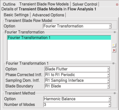
Typically, one mode is sufficient for a blade flutter calculation; however, for some transonic flow regimes, three modes may be required to accurately resolve the flow.
In the Solver Control details view, on the Basic Settings tab, ensure that Transient Scheme > Option is set to
Harmonic Balance, specify the maximum number of iterations (Max. Iterations), and set the pseudo-time step size (Fluid Timescale Control settings). Typically, the size of the pseudo-time step (Physical Timescale) is equal to the period of the vibration cycle divided by the intended number of pseudo-time steps per period.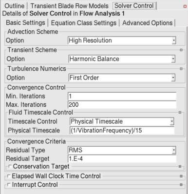
The period of the vibration cycle is equal to 1/(vibration frequency). A typical number of pseudo-time steps per cycle is between 15 and 30. Recall that the lower the number of pseudo-time steps that can be used while maintaining a stable solution, the more efficient the calculation is with respect to the time marching method.
The Mesh Deformation option cannot be set to
Periodic Regions of Motion. For details on thePeriodic Regions of Motionoption, see Periodic Regions of Motion.
The Harmonic Forced Response analysis requires two inputs from the CFD analysis. They are the forcing function due to the unsteady pressure, and the contributions to the aerodynamic damping matrix. In both cases, the information is required in the form of the first harmonic of the surface pressure field on the blade being analyzed. For details, see Harmonic Analysis in the Theory Reference.
The forcing function in the Harmonic Forced Response analysis is obtained from transient blade row interactions, while the contributions to the aerodynamic damping matrix is obtained from the blade flutter analysis. You can use either a full-wheel model or a reduced geometry using the Time-Transformation or Fourier-Transformation methods as a pitch-change model. These unsteady pressure values will be exported in the complex form obtained from their Fourier representation. In order for the solver to complete these calculations, you must specify the excitation frequency. The excitation frequency can be specified as an engine order or obtained from the blade vibration frequency. For details, see [Export Surface Name]: Excitation Frequency in the CFX-Pre User's Guide.
The engine order represents the number of disturbances (or pulses) per revolution.
Therefore, the excitation frequency can be computed as  , where
  is the excitation frequency,
  is
the engine order, and
is
the engine order, and  is the angular velocity of the machine.
For blade flutter cases that have the Periodic Displacement mesh motion option, the CFX-Solver writes the passage number to the field data of the exported data.
If the periodic mesh displacement input vector components are specified using
Cartesian Components, then the CFX-Solver will export a profile file that contains both the nodal diameter and mode multiplier, where the value of the mode multiplier is the same asScaling.If the periodic mesh displacement input vector components are specified using
Normalised Cartesian Components, then:In a new case, the CFX-Solver will export a profile file that contains both the nodal diameter and mode multiplier, where mode multiplier is defined as
Amplitude/Maximum Displacement.In an existing case that was made from a release earlier than Release 18.0, the CFX-Solver will export a profile file that does not contain the mode multiplier. However, an existing case can be upgraded as follows:
With the case loaded in CFX-Pre, edit the boundary that has periodic mesh displacement (so that its details view appears).
If the existing case was made from a release earlier than Release 17.2, select the Use Profile Data option (and, if there is more than one profile, select the applicable profile).
Click Apply.
This updates the case in CFX-Pre by adding the required CCL.
Save the case file (and/or write the solver input file).
Note that if the above procedure is not followed, the maximum displacement will not be in the solver input file, and the exported profile file will not contain the mode multiplier.
Note: CFX can export profile data to the mesh coordinates used by Ansys Mechanical. For details, see Mapping Profile Data to a File in the CFX-Pre User's Guide.
Note: When exporting complex pressures on a boundary with mesh motion (for example, a Fourier Transformation blade flutter case), the results will be exported using the initial mesh coordinates from the CFX-Solver run.
Note: CFX and Mechanical use different representations for harmonic pressure
loads,  , where pressure
  is a function of time
  .
.
CFX represents harmonic pressure loads using real-number Fourier coefficients as:
 | (6–3) |
where  represents the index of the mode,
  represents the total number of
modes,
represents the total number of
modes,  and
and  represent the real-number Fourier coefficients, and
  represents the base
frequency.
represents the base
frequency.
In contrast, Mechanical represents harmonic pressure loads using imaginary and real pressure components as:
 | (6–4) |
where  and
and  represent the real and imaginary pressure components, respectively, of the
contribution for mode
represent the real and imaginary pressure components, respectively, of the
contribution for mode  , and
, and  represents the real, time averaged, value.
By comparing Equation 6–3 and Equation 6–4, it can be seen that  is analogous to
  ,
while
,
while  is analogous to
  .
.
When exporting to Mechanical, CFX exports  and
and  .
.
For more details, see Harmonic Analysis in the Theory Reference.
Ansys CFX enables you to use Time-Transformation Transient Rotor Stator interfaces to model multistage turbomachinery configurations. In general, the Time Transformation method is used for small-to-moderate pitch-change, multistage turbomachines. Note that the Time Transformation method cannot be used with incompressible cases. The Time Transformation method is not recommended when the rotation rate of the rotor is very low.
The multistage modeling capability of the Time Transformation method in Ansys CFX is demonstrated by the examples in the following sections.
- 6.1.8.5.1. Modeling a Single-pitch-ratio Multistage Turbomachine using the Time Transformation Method
- 6.1.8.5.2. Modeling 1.5 Stages with Two Different Pitch Ratios using the Time Transformation Method
- 6.1.8.5.3. Modeling a multistage turbomachine with Time Transformation TRS and other interfaces: Profile Transformation & Stage
- 6.1.8.5.4. Modeling a multistage turbomachine with Time Transformation TRS and single-sided Time Transformation interfaces (STT-TRS)
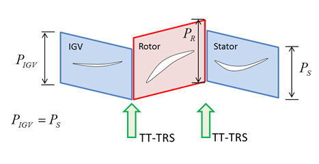
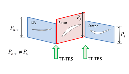
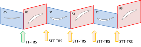
In this special situation, where every other row of the turbomachine has same number of blades, we have technically the configuration of a single disturbance being imposed in each passage. Therefore, there is only one pitch ratio present in the configuration. An example of such a case would be a machine in which all stator rows have the same number of blades and all rotors rows have the same number of blades, but the number of blades differs between the stator rows and the rotor rows. This special case can be modeled accurately by using TT correction on all the TRS interfaces (TT-TRS) between rows. Figure 6.8: 1.5 stage machine with equal number of blades in rows 1 & 3 but different than in row 2. Flow can be accurately modeled via a sequence of TT-corrected TRS interfaces. demonstrates an example of a 1.5 stage turbomachine with an equal number of blades in the first and third rows, but a different blade count in the middle row. TT-TRS interfaces have been applied sequentially to this configuration.
To set up this case:
Set the two rotor/stator interfaces (in the example of Figure 6.8: 1.5 stage machine with equal number of blades in rows 1 & 3 but different than in row 2. Flow can be accurately modeled via a sequence of TT-corrected TRS interfaces., the IGV/Rotor and the Rotor/Stator interfaces) as Transient Rotor Stator (TRS).
In the Outline tree view, edit the
Transient Blade Row Modelsobject under the applicable flow analysis.Create two disturbances of the same type (TT) and assign each of them to the respective TRS interfaces created in step 1.
Figure 6.8: 1.5 stage machine with equal number of blades in rows 1 & 3 but different than in row 2. Flow can be accurately modeled via a sequence of TT-corrected TRS interfaces.
This modeling method will allow for capturing accurate blade passing signals in all the rows as well as obtaining accurate machine performance. The limitation on acceptable pitch ratio with use of the TT method still applies to this modeling technique.
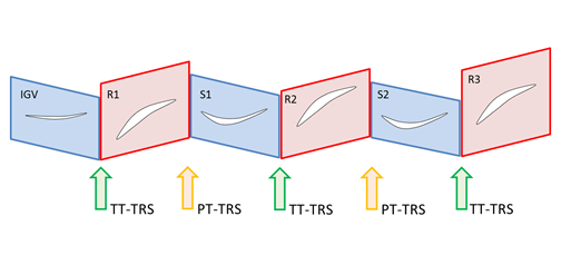
In this configuration, each row has a different pitch value or two distinct pitch ratios across the machine, as shown in the following figure. The Time Transformation TRS interface can also be applied sequentially between the IGV and Rotor, and between the Rotor and Stator. This extension of the Time Transformation TRS interface allows for capturing both upstream and downstream blade passing frequencies in the rotor passage, making this modeling method useful for forced response analysis.
Figure 6.9: 1.5 stages with differing blade numbers between rows 1, 2 & 3. Flow can be modeled via a sequence of TT-TRS interfaces.
The following procedure is necessary to model a 1.5 stage turbomachine with two different pitch ratios:
Set all the rotor/stator interfaces to be of the TRS type.
In the Outline tree view, edit the
Transient Blade Row Modelsobject under the applicable flow analysis.Create Time Transformation disturbances for each of the TRS interfaces that are corrected by Time Transformation.
This modeling strategy will allow for obtaining accurate machine performance as well as capturing blade passing signals in rows 1 and 2. On the other hand, row 3 may contain polluted frequency content due to modeling approximation. The limitation on acceptable pitch ratio with use of the Time Transformation method still applies to this modeling technique.
Important: It is not recommended that you use Time Transformation TRS for every rotor-stator interface beyond a 1.5 stage configuration. For turbomachines with more than 1.5 stages, we recommend the modeling strategy shown in Modeling a multistage turbomachine with Time Transformation TRS and other interfaces: Profile Transformation & Stage.
Accurate multistage performance can be predicted by using a combination of Time Transformation TRS and other interface models such as Profile Transformation TRS or Stage interface (mixing-plane). For maximum accuracy, it is recommended that you use Time Transformation TRS at each rotor passage inlet, and a Profile Transformation TRS or Stage interface at the rotor passage outlet. The idea is to minimize modeling error at the TRS interfaces where flow shocks might be crossing by using Time Transformation TRS modeling at those interfaces. The next two figures illustrate two common possible combinations of interfaces for modeling multistage configurations.
Figure 6.10: Multistage modeled with a combination of TT and PT interfaces. For high speed flows, the TT-TRS interfaces should be placed where shocks are crossing between the adjacent passages. This is typically happening at the interface between the exit of the stator row and the inlet of the rotor row.
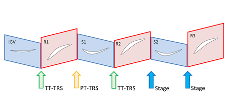
The following procedure is necessary to model multistage turbomachines with Time Transformation and Profile Transformation interfaces:
Set all the rotor/stator interfaces to be of the TRS type.
In the Outline tree view, edit the
Transient Blade Row Modelsobject under the applicable flow analysis.Create Time Transformation disturbances for the TRS interfaces that are corrected by Time Transformation.
This modeling strategy will allow for obtaining accurate machine performance for turbines and compressors. However, this modeling strategy is not intended to be used for capturing accurate blade passing signals throughout the machine due to the modeling approximation of the Profile Transformation method. The limitation on acceptable pitch ratios using the Time Transformation method still applies to this modeling technique.
For multistage machines, an alternative to using PT-TRS or TT-TRS models on both sides of TRS interfaces is to apply the so-called single-sided TT interface (STT-TRS). The STT-TRS interface model applies the PT model to one side of the interface (typically the upstream side) and the TT model to the other side (typically the downstream side).
Also, you can reverse this correction if necessary (for example, if you want to capture signals from the downstream component). The advantage of using STT-TRS over PT-TRS is that STT-TRS maintains the upstream blade wake thickness as it convects downstream. This modeling strategy results in more accurate accounting of machine performance and losses.
For maximum accuracy, it is recommended that you use TT-TRS at the rotor passage inlet and STT-TRS on the rotor passage exit. Figure 6.12: Multistage modeled with combination of TT-TRS and STT-TRS interfaces illustrates how the STT-TRS is used with TT-TRS in modeling a multistage machine.
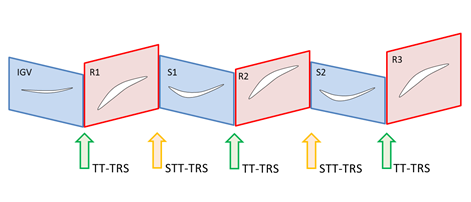
It is also possible to apply sequentially several STT interfaces, as shown in Figure 6.13: Multistage modeled with several STT-TRS interfaces in sequence.
The following procedure is necessary to model multistage turbomachines with TT-TRS and STT-TRS interfaces:
Set all the rotor/stator interfaces to be of the TRS type.
In the Outline tree view, edit the
Transient Blade Row Modelsobject under the applicable Flow Analysis object.Create TT disturbances for all of the TRS interfaces that are corrected by either TT or STT.
For the STT-TRS interfaces, the TT disturbances have to be modified on one of the domain interface sides. On the side of the interface not modeled by TT (the PT side as explained above), the side option should be changed to
None. The setting for the other side can be left as it is; the TT model will be applied to that side. Note that the interface side name is displayed in the transient rotor stator domain interface’s Basic Settings tab.
This modeling strategy can improve the accuracy of machine performance predictions for both turbines and compressors. However, this type of modeling is not intended for capturing accurate blade passing signals throughout the machine due to the modeling approximation of the STT-TRS method. The limitation on acceptable pitch ratio with use of the TT method still applies to this modeling technique.
The Fourier Transformation Transient Rotor Stator (FT-TRS) interface can handle flow cases in which an impeller or rotor is attached to a full 360° domain, where the impeller or rotor may experience extremely large inflow variation, such as a once-per-revolution or three-per-revolution inflow disturbance.
Note: An FT-TRS interface enables the modeling of just two impeller or rotor blades connected to the full 360° domain. There is little or no benefit in using the FT-TRS interface in this way for cases that involve a small number of impeller or rotor blades.
The following cases are discussed:
In this case, the impeller experiences a long-period disturbance due to the asymmetry of the volute.
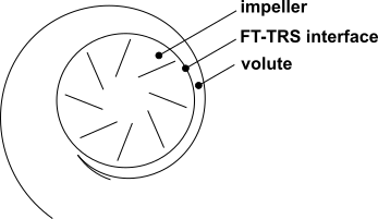
To set up an impeller in a vaneless volute:
Specify the FT-TRS interface as the interface between the volute and the blade passages.
Create a disturbance of type
Rotor Stator:On the impeller side, select
Phase
                                          Corrected
and then select the phase-corrected and sampling interfaces (which are between impeller blades).On the volute side, select
None.The side of the FT-TRS interface that is attached to a 360° sector will have neither a sampling domain interface nor a phase corrected interface.
The disturbance accounts for the signal from the volute.
Note that a similar procedure could be used to set up a case involving a fan in a crosswind.
In this case, the impeller experiences two flow disturbances: one short-period disturbance due to the vanes; one long-period disturbance due to the asymmetry of the volute.
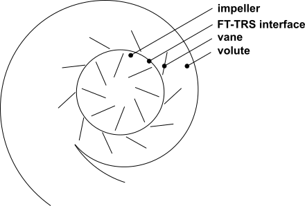
To set up an impeller in a vaned volute:
Follow the steps for a vaneless volute.
Because of the presence of the vanes, the disturbance is automatically configured to account for the signal from the vanes.
To account for the signal from the volute, create a (second) disturbance of type
Rotational Flow Boundary Disturbance:On the impeller side, select
Phase
                                          Corrected
and then select the phase corrected and sampling interfaces (which are between impeller blades).Specify that the number of passages in 360° (under the external passage definition) is one, to capture the once-per-revolution disturbance of the volute.
Set the Signal Motion option to
Stationaryto indicate that the signal comes from the volute side of the Rotor Stator interface.