VM199

VM199
Oil Film Bearing Supporting a Rotating Shaft and Subjected to a Static Load

Overview

Reference:

Friswell, M.I., Penny, J.E.T., Garvey, S.D., Lees, A.W., Dynamics of Rotating Machines, Cambridge University Press, 2010, pg. 181

Analysis Type(s):

Static Analysis (ANTYPE = 0)

Transient Analysis (ANTYPE = 4)

Element Type(s):

3D Structural Mass Element (MASS21)

2D Spring-Damper Bearing Element (COMBI214)

3D 8-Node Structural Solid (SOLID185)

3D 8-Node Surface-to-Surface Contact (CONTA174)

3D Target Segment (TARGE170)

3D Hydrodynamic Bearing Element (FLUID218)

Input Listing:

vm199.dat

Test Case

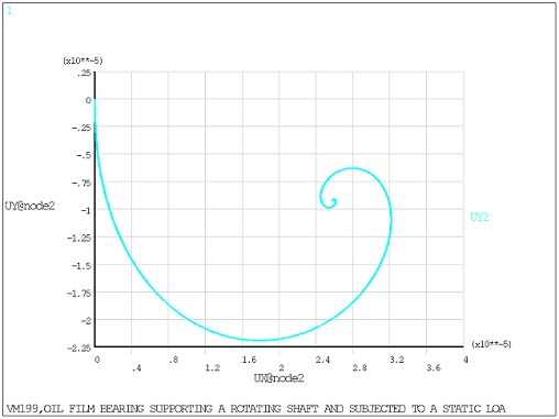
An oil film bearing defined by its radial clearance, diameter, and length supports a rotating shaft and is subjected to a static vertical load of 525 N. Calculate the bearing eccentricity ratio and the bearing coefficients under these conditions.

Material Properties

Geometric Properties

Mass of the shaft, m = 53.51683 kg

Viscosity of the oil = 0.1 Pa˙S

Radial clearance, x_clear = 1.0 x 10^-4

Length, l = 0.03 m

Radius, r = 0.05 m

Shaft rotational velocity, ω = 1500 RPM

Acceleration due to gravity, g = 9.81 m/sec² in order to apply a vertical static load of F = mg = 525 N

Perturbation increment = 1.0 x 10^-5

Analysis Assumptions and Modeling Notes

A simplistic bearing-shaft model is created using:

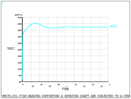
For the 2D model: COMBI214 and MASS21 elements. The bearing geometry is defined via COMBI214 constants.
For the 3D model: FLUID218 and SOLID185 elements. The bearing geometry is defined via FLUID218 real constants and material property.

Nonlinear transient analysis is first performed on the model with an end time of 0.20 seconds (5 cycles)

For the 2D model, a time increment of 1.0 x 10^-4 seconds is set to determine the shaft equilibrium position and eccentricity ratio. The shaft rotational velocity in rad/sec is specified using nodal constraint (D,,OMGZ).

The shaft equilibrium position obtained from transient analysis, along with a small perturbation increment, is used in a static analysis to determine the bearing stiffness and damping coefficients:

For the 2D model: The shaft equilibrium position is input via the D command and the perturbation increment is input via COMBI214 real constants. The shaft rotational velocity in rad/sec is specified via the OMEGA command in the linear static solve.
For the 3D model: The shaft equilibrium position is input via FLUID218 real constants. A small perturbation (1E-6) is given about the equilibrium position and the bearing forces are calculated. Using these bearing forces, the stiffness and damping characteristics are evaluated.

Results Comparison

2D	Units	Target	Mechanical APDL	Ratio
Eccentricity Ratio	-	0.266	0.275	0.969
KXX	MN/m	12.810	12.567	1.019
KYY	MN/m	8.815	8.712	1.012
KXY	MN/m	16.390	15.818	1.036
KYX	MN/m	-25.060	-24.433	1.026
CXX	kNs/m	232.900	225.410	1.033
CYY	kNs/m	294.900	287.068	1.027
CXY	kNs/m	-81.920	-80.406	1.019
CYX	kNs/m	-81.920	-80.461	1.018

Figure 307: 2D Shaft Orbit Plot

Figure 308: 2D Maximum Fluid Pressure

3D	Units	Target	Mechanical APDL	Ratio
KXX	MN/m	12.810	12.139	1.055
KYY	MN/m	8.815	8.017	1.100
KXY	MN/m	16.390	15.910	1.030
KYX	MN/m	-25.060	-24.210	1.035
CXX	kNs/m	232.900	224.511	1.037
CYY	kNs/m	294.900	285.459	1.033
CXY	kNs/m	-81.920	-76.167	1.076
CYX	kNs/m	-81.920	-84.654	0.968

Figure 309: 3D Pressure Solution