The frequency-sweep method computes the harmonic solution in the middle of the requested frequency range and then interpolates the matrices and loading across the given range. The procedure to use this method for harmonic analysis is similar to the full method:
Applying Loads and Obtaining the Solution (Choose VT on the HROPT command.)
The frequency-sweep method performs accurate approximations of the results across the frequency range in user-specified steps.
If the loading, material properties, or real constants defined with a data table are frequency-dependent (for example, tabular input on the BF, command, material data defined via the TBFIELD command, or tabular real constant data defined for element COMBIN14) and too few data points exist in the table, the polynomial interpolation of the values will be poor. In case of abrupt variations for a given frequency f2, Ansys, Inc. recommends splitting the frequency range [f1 f3] into two ranges (for example, [f1 f2]; [f2 f3]) and performing separate analyses on each range.
See also these topics on the frequency-sweep method:
The frequency-sweep method supports frequency-dependent material elastic properties and efficiently computes the frequency response over an entire frequency range.
Frequency-dependent material properties can be used with the following elements:
| Element | Frequency-Dependent Material Properties (defined using TB,ELAS and TB,SDAMP,,,,STRU commands) |
|---|---|
| PLANE182 | EX, STRU |
| PLANE183 | EX, STRU |
| SOLID185 | EX, STRU |
| SOLID186 | EX, STRU |
| SOLID187 | EX, STRU |
| SOLID272 | EX, STRU |
| SOLID273 | EX, STRU |
| SOLID285 | EX, STRU |
Be sure to use the hysteretic damping formulation of the HROPT
command (DAMP = HYST). For more information, see the
documentation for the TB,ELAS and
TB,SDAMP,,,,STRU commands.
If you define the damping ratio (TB,SDAMP,,,,STRU) as a linear function of the frequency, the damping exhibits behavior similar to that of viscous damping. For more information about the hysteretic and structural damping formulations, see Viscous or Hysteretic Damping in the Theory Reference.
Limitations
The frequency-dependent tables (defined by the TB,ELAS and TB,SDAMP commands) define piecewise linear functions. These are used to define the stiffness and damping matrices, which in turn are fitted with a polynomial over the entire frequency range to compute their derivatives as a function of frequency. Therefore, if the piecewise linear approximation of the material properties is too coarse, the results will be poor.
Consider a cantilever beam with a Young's modulus of 20x106 psi for static conditions and 30x106 at 500Hz.
The following input demonstrates use of the frequency-sweep harmonic analysis to solve this problem:
ETYPE=186
LF = 10               ! Starting frequency
UF = 500              ! Ending frequency
N = 50                ! Number of substeps
/PREP7
!*
ET,1,ETYPE
/com, * ==============================================
/com, *
/com, *    frequency-dependent material properties
/com, *
/com, * ==============================================
TB,ELASTIC,1,,2      ! Elastic data table
TBFIELD, FREQ,1     ! First frequency value
TBDATA,1,20e6,0.3    ! E and m
TBFIELD,FREQ,500    ! Fifth frequency value
TBDATA,1,30e6,0.3
TB,SDAMP,1,,1       ! Damping data table
TBFIELD,FREQ,1     ! First frequency value
TBDATA,1,0.02       ! Damping coefficient
TBFIELD,FREQ,500     ! Fifth frequency value
TBDATA,1,0.01
MP,DENS,1,.10
BLOCK,0,10,0,2,0,2
LSEL,S,LOC,X,-.5,0.5
LESIZE,ALL,,,2
LSEL,S,LOC,X,9.5,10.5
LESIZE,ALL,,,2
LSEL,S,LOC,X,2,8
LESIZE,ALL,,,5
VMESH,ALL
FINISH
/SOL
LSEL,S,LOC,X,-.5,0.5
DL,all,,all
KSEL,S,LOC,X,8,12
KSEL,R,LOC,Y,-.5,.5
FK,ALL,FY,1000
ASEL,S,LOC,Y,1.8,2.2
SFA,ALL,,PRES,1000,
allsel
FINI
/com, * ==============================================
/com, *
/com, *       Frequency-Sweep Harmonic Analysis
/com, *
/com, * ==============================================
/SOLU
ANTY,HARM
HROUT,OFF       ! Print complex displacements as amplitude and phase angle
KBC,1
HROPT,VT,,,,HYST
harfrq,LF,UF
nsubst,N
Solve
FINISH
/post26
nsol,10,57,u,y,d1
prvar,10
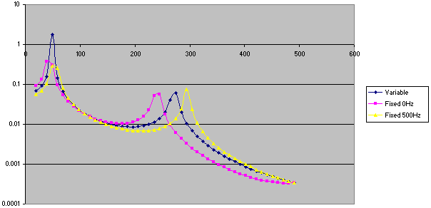
The following figure shows the difference in the Y displacement at the end of the beam, taking constant material properties for 0 Hz, constant properties for 500 Hz, and variable properties:
Because of the frequency step used to create the frequency response, the first peak is higher on the variable curve than the other two.


