


Any constraints other than multistage cyclic and interstage constraints are additional constraints. This section covers application of loads and additional constraints. In general, all loads and additional constraints must be applied to both the base and duplicate sectors. The duplication is not done automatically during the solve.
Additional constraints must be applied to the base and duplicate sectors. Any non-zero constraints will have a cyclic behavior within the stage. Constraints cannot be applied to the cyclic or interstage boundaries. The one notable exception is that you can fix all degrees of freedom on the cyclic boundaries (D,,ALL).
Constraint and joint elements (MPC184) can be used in a multistage model with the following limitations:
They are not permitted at the cyclic edges (including the cyclic axis) or at interstage boundaries.
One MPC184 element can only be attached to a single stage or multiharmonic stage group.
If you use multipoint constraint (MPC) contacts inside a stage, set KEYOPT(9) = 1 (exclude initial penetration or gap and offset). Otherwise, these could lead to non-zero constant terms in the contact element internal constraint equations. These terms are not compatible with constraints (D) that are internally applied on the duplicate sector when it is not needed in the analysis.
Remote loads and displacements can be applied to a multistage model. The recommendations and limitations for applying remote loads and displacement follow the same guidelines as those for cyclic symmetry (see Loading Considerations in the Cyclic Symmetry Analysis Guide). Specific to multistage analyses, note that a single pilot node may only attach to the target elements on one stage. To apply additional loads or constraints to another stage, you must define an additional pilot node and create target elements on that stage.
During each multistage solve, just like any other solve, any user-defined constraint equations (CE, CEINTF,...) may be altered. For each additional solve (SOLVE), remove these constraints (CEDELE) and reissue them (CE, CEINTF,…).
Loads can be applied to each stage. If you apply loads using additional elements such as surface effect elements (see SURF elements in the Element Reference), those elements must be included in the appropriate stage components (MSOPT,NEW).
Loads are not permitted at the cyclic or interstage boundaries.
Body loads such as rotational velocity (OMEGA) should only be applied to the HI = 0 stage to maintain the expected cyclically symmetric load in static analyses. See Static Loading for more details.
There is no automatic transfer of loads from the base sector to duplicate sectors or stage clones. Loads must be applied as needed for a given loading scenario to both the base and duplicate sector (if it exists) and stage clones if multiple harmonics are present. There are two exceptions to this:
When a tabular load having node number (NODE) or element number (ELEM) as the primary variable is applied to a harmonic index 0 base sector in a static analysis, the tabular loads are automatically copied to the harmonic index 0 duplicate sector and all of the harmonic index 0 base and duplicate sectors of secondary harmonic stage clones in a multiharmonic group.
When a tabular load includes the multistage harmonic index (MSHI) as a primary variable, the tabular loads are automatically replicated to generate a traveling wave (engine order) load as detailed in the next section.
You can apply loads or boundary conditions using a harmonic index (HI)-based table to eliminate the need to copy loads from the base sector to duplicate sectors or stage clones. To create an HI-based table, include MSHI as a primary variable. If you have defined multiple harmonic indices for the MSHI variable in an HI-based table, there may be unique table copies to multiple stages. The program does not directly copy loads from an HI-based table. Instead, it copies real and imaginary loads or boundary conditions in a manner that creates a typical traveling wave (engine order) load for the harmonic index specified.
HI-based tables must conform to the following requirements:
You must specify and explicitly apply both a real and an imaginary HI-based table. Even if the real or imaginary load has a value of zero, it still must be applied explicitly by creating the real or imaginary HI-based table.
Applying loads or boundary conditions using HI-based tables results in additional table creation during the solution step. For this reason, an HI-based table should not be reused unless the original table and all duplicates of the original table are deleted.
You cannot specify a harmonic index in an HI-based table that is applied to a multiharmonic group that is smaller than the HI of the group's lead harmonic stage. For example, you cannot apply an HI-based tabular load with HI = 1 to a multiharmonic group if its lead harmonic stage is HI = 2.
If you are applying an HI-based tabular load with a single HI to a stage that has only one HI, they must be equal.
At least one harmonic index in the table must be represented in the stage to which it is applied.
The example snippet and selected output are presented here to demonstrate HI-based table creation and subsequent load application.
! Two multiharmonic stage groups
! Each group has a HI = 1 and HI = 5 stage
HI1 = 1
HI1_2 = 5
HI2 = 1
HI2_2 = 5
msopt,modify,stage1,HI1
cecycms
msopt,modify,stage1_2,HI1_2
cecycms
msopt,modify,stage2,HI2
cecycms
msopt,modify,stage2_2,HI2_2
cecycms
….
! Table has 3 dimensions: Time, Node, MSHI
nTime = 2     ! 2 Time points
nNode = 2     ! 2 Nodes
nMSHI = 2     ! 2 Harmonic indices
*DIM,force_re,TABLE,nTime,nNode,nMSHI,TIME,NODE,MSHI
*taxis,force_re(1,1,1),1,0,1.0
*taxis,force_re(1,1,1),2,519,521
*taxis,force_re(1,1,2),2,519,521
*taxis,force_re(1,1,1),3,1,5             ! Harmonic index 1 and 5
*do,i,1,nTime
     *do,j,1,nNode
            force_re(i,j,1) = (j*1.0e+3) ! Harmonic index 1
            force_re(i,j,2) = (j*1.4e+3) ! Harmonic index 5
     *enddo
*enddo


*DIM,force_im,TABLE,nTime,nNode,nMSHI,TIME,NODE,MSHI
*taxis,force_im(1,1,1),1,0,1.0
*taxis,force_im(1,1,1),2,519,521,523
*taxis,force_im(1,1,2),2,519,521,523
*taxis,force_im(1,1,1),3,1,5             ! Harmonic index 1 and 5
*do,i,1,nTime
     *do,j,1,nNode
            force_im(i,j,1) = (j*10)     ! Harmonic index 1
            force_im(i,j,2) = (j*120)    ! Harmonic index 5
     *enddo
*enddo
nsel,s,node,,519,521,2
f,all,fz,%force_re%,%force_im%           ! Apply real and imaginary tables as nodal force

…

Solve   !  the solve command triggers the internal table copies

…

! View input tables
*stat,force_re,0,,0
*stat,force_im,0,,0

! View list of tables created
*stat,all

! List the load
flist
Output from this snippet illustrates load application using the HI-based tables. The original real and imaginary tables are listed first, showing the different loads for both harmonic index 1 and 5.
PARAMETER STATUS- FORCE_RE  (     43 PARAMETERS DEFINED)
                  (INCLUDING        7 INTERNAL PARAMETERS)

      LOCATION                VALUE
        0       0       1    1.00000000
        1       0       1    0.00000000
        2       0       1    1.00000000
        0       1       1    519.000000
        1       1       1    1000.00000
        2       1       1    1000.00000
        0       2       1    521.000000
        1       2       1    2000.00000
        2       2       1    2000.00000
        0       0       2    5.00000000
        1       0       2    0.00000000
        2       0       2    0.00000000
        0       1       2    0.00000000
        1       1       2    1400.00000
        2       1       2    1400.00000
        0       2       2    0.00000000
        1       2       2    2800.00000
        2       2       2    2800.00000

      PRIMARY VARIABLE(S): 1=TIME 2=NODE 3=MSHI

 PARAMETER STATUS- FORCE_IM  (     43 PARAMETERS DEFINED)
                  (INCLUDING        7 INTERNAL PARAMETERS)

      LOCATION                VALUE
        0       0       1    1.00000000
        1       0       1    0.00000000
        2       0       1    1.00000000
        0       1       1    519.000000
        1       1       1    10.0000000
        2       1       1    10.0000000
        0       2       1    521.000000
        1       2       1    20.0000000
        2       2       1    20.0000000
        0       0       2    5.00000000
        1       0       2    0.00000000
        2       0       2    0.00000000
        0       1       2    0.00000000
        1       1       2    120.000000
        2       1       2    120.000000
        0       2       2    0.00000000
        1       2       2    240.000000
        2       2       2    240.000000
The following variable listing shows all of the tables, including those created internally. Note that table copies were made to the 3rd and 4th stages in order of definition (see the order based on the MSOPT command in the snippet) because the nodes related to the table were only associated with stage 3. The copies were made to the duplicate sector of stage 3 and the base and duplicate sector of the other stage harmonic in the multiharmonic group (stage 4).
NAME                                           VARIABLE(S)
 FORCE_IM                                       1=TIME 2=NODE 3=MSHI
 FORCE_IM_STID3_DUP                             1=TIME 2=NODE 3=
 FORCE_IM_STID4                                 1=TIME 2=NODE 3=
 FORCE_IM_STID4_DUP                             1=TIME 2=NODE 3=
 FORCE_RE                                       1=TIME 2=NODE 3=MSHI
 FORCE_RE_STID3_DUP                             1=TIME 2=NODE 3=
 FORCE_RE_STID4                                 1=TIME 2=NODE 3=
 FORCE_RE_STID4_DUP                             1=TIME 2=NODE 3=
The load listing shows that the loads were indeed copied to the nodes associated with stage 3 duplicate sector and stage 4 base and duplicate sectors. The load that is copied to the duplicate is multiplied by -i, where i is the unit imaginary number.
NODE  LABEL     REAL           IMAG
      519  FZ      1000.00000      10.0000000
      521  FZ      2000.00000      20.0000000
      625  FZ      10.0000000     -1000.00000
      627  FZ      20.0000000     -2000.00000
      731  FZ      1400.00000      120.000000
      733  FZ      2800.00000      240.000000
      837  FZ      120.000000     -1400.00000
      839  FZ      240.000000     -2800.00000
You can apply harmonic backward traveling wave (BTW) and forward traveling wave (FTW) loads directly to your model. The following summary table describes the procedure depending on if your model is a 360 (full non cyclic) model, a single stage cyclic model, or a single stage cyclic superelement model[a].
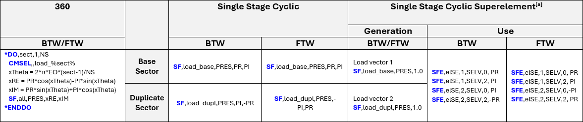
aSee details on applying an imaginary force vector in Applicable Loads in a Substructure Analysis in the Substructuring Analysis Guide.
where
| EO is the engine order excitation. Note that EO is positive for BTW and negative for FTW. |
| NS is the number of sectors. |
| load_xx is the component of elements in sector xx on which the load is applied. |
| PR is the real component of the pressure load. |
| PI is the imaginary component of the pressure load. |
| load_base is the component of base sector nodes at which pressure load is defined. |
| load_dupl is the component of duplicate sector nodes at which pressure load is defined. |
| elSE is the element number of the superelement. |