


A far-field element, also called an infinite boundary element, allows you to model the effects of far-field decay in magnetic, electrostatic, thermal, or electric current conduction analyses. Without far-field elements, you otherwise model the near-field to a distance where you assume you can apply a flux-parallel or flux-normal boundary condition. Such an assumption is an approximation, however, that can significantly affect the accuracy of the results in the near-field area of the model. Using far-field elements, you are not forced to make assumptions about conditions at the model boundary. The elements model the decaying behavior of the field, out to an infinite distance, even though the elements themselves extend to a finite distance. They produce better accuracy, often at a computation reduction in the size of the model.
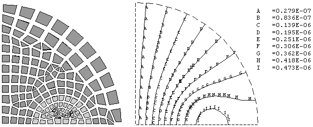
Consider, for example, a dipole and its 2D, quarter-symmetry finite element model (see Figure 11.1: Flux Lines Without Far-Field Elements). Without far-field elements, you should model the air surrounding the iron core out to a very large distance where the assumption of a flux-normal boundary conditions is reasonably correct. The number of elements required, and the corresponding computational expense, means you'll trade off some accuracy for smaller model size. Note the imposed flux-normal behavior at the boundary.
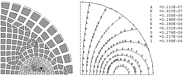
The alternative shown below uses one-dimensional (line) far-field elements at the boundary instead of the flux-normal condition. Without extending the physical location of the model boundary, the behavior of the flux lines at the boundary is much more realistic, and the results in the near-field are better as a result.
Mechanical APDL offers 2D and 3D solid infinite elements for far-field effects.
How much of the surrounding air should you model? The answer depends on the problem you are solving. For relatively closed flux paths (little leakage to surroundings), not much of the air needs to be modeled, that is, you can place the far-field elements relatively close to the model region of interest. For open-boundary problems, you should extend the air elements well beyond the region of interest before placing the far-field elements.
Far-Field Elements Described
Mechanical APDL offers the following far-field elements.
Table 11.1: 2D Far-Field Elements
| Element | Description | Analysis Category | Enclosed Elements | Analysis Type |
|---|---|---|---|---|
| INFIN110 |
4 or 8 Node Quadrilateral Planar or Axisymmetric Models | Magnetic |
Static Harmonic Transient | |
| Electrostatic |
Static Harmonic | |||
| Thermal |
Steady-state Transient | |||
| Electric Current Conduction |
Steady-state Harmonic Transient |
Table 11.2: 3D Far-Field Elements
| Element | Description | Analysis Category | Enclosed Elements | Analysis Type |
|---|---|---|---|---|
| INFIN47 |
4 Node Quadrilateral or 3 Node Triangle | Magnetic |
Static Harmonic Transient | |
| Thermal |
Steady-state Transient | |||
| INFIN111 |
8 or 20 node hexahedral | Magnetic |
Static | |
| Electrostatic |
Static Harmonic | |||
| Thermal |
Steady-state Transient | |||
| Electric Current Conduction |
Steady-state Harmonic Transient |
Note: You can also use far-field elements in a thermal analysis. Refer to the Thermal Analysis Guide for details on thermal analysis.