The program GUI includes an intuitive hierarchical tree structure interface for defining many material models. A logical top-down arrangement of material categories guides you in defining the appropriate model for your analysis.
Not all material models are available via the GUI. For more information, see GUI-Inaccessible Material Properties in the Material Reference.
For more information on individual material models, see the Material Reference.
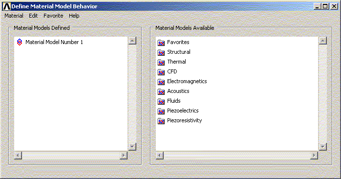
Access the material model interface via . The Define Material Model Behavior dialog box appears, which originally displays the top level of the tree structure:
The Material Models Available window on the right displays a list of material categories (for example, Favorites, Structural, Thermal, Electromagnetics).
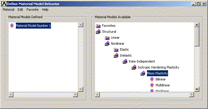
If a category is preceded by a folder icon, there are subcategories available under the main category. When you double-click the category, the subcategories appear indented and below the category:
For example, under Structural are categories Linear, Nonlinear, and others. The models are further categorized so that you will eventually see a vertical list of material property sets or material models that are included under that category (for example, under von Mises Plasticity are: Bilinear, Multilinear, and Nonlinear). When you have decided which material property set or model to use, choose it by double-clicking on the item. A dialog box appears that prompts you for the required input data for that particular model or property set. Details of a data input dialog box are presented in Entering Material Data.
A Material Favorite is a template of material properties. It is used as a short cut to frequently used properties, instead of navigating through the detailed tree structure each session. You can create a named template based on a currently defined material model through .You can also delete a named template through the menu. For any consecutive sessions, you will then be able to access this named template in the Favorites folder shown in the Material Models Available window.
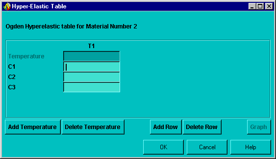
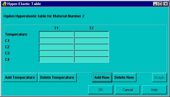
Included in a data input dialog box is a table whose rows and columns you can alter depending on the requirements of the specific material property or model you have chosen. A typical data input dialog box is shown below:
There are two interaction areas within a material data input dialog box: the data input table, and a series of action buttons that appear at the bottom. Depending on the material item you are defining, the labels in the table vary, as do the number of rows and columns that appear initially. The material item also dictates the number of rows and columns that you are allowed to add or delete. In most cases, the columns represent temperatures, and the rows represent data values (for example, density as a linear isotropic property, or constants for a particular nonlinear model).
Temperature Dependent Data
Initially, the table is set up for temperature independent data so the temperature field is grayed out. At this point, should you decide to enter data for various temperatures, you can quickly add columns of text fields for the data representing each temperature. You can add or delete the temperature dependent data at any time. You do not need to predetermine if the data should be temperature dependent.
Adding and Deleting Columns
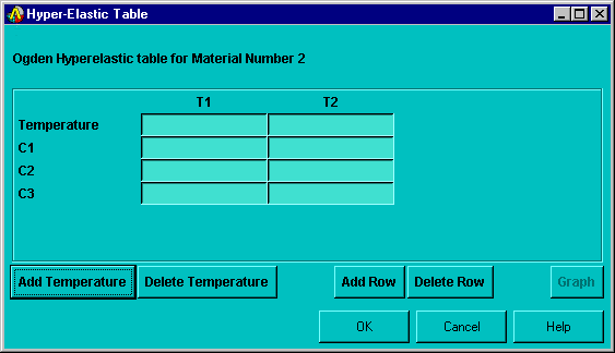
To add a column, position the text cursor in any field in the existing column, then click the button. A new column appears to the right of the existing column, and both temperature fields become active, as shown below:
You then enter the two temperatures and the associated data in the rows. You can add more temperature columns, as needed, by following the same procedure. You can insert columns between existing columns by clicking the text cursor in a field within a column that is to the left of where you want to insert the new column, then clicking on the button.
You can delete a temperature column by positioning the text cursor in any field within the column, and clicking on the button.
Adding and Deleting Rows
You may have the need to add another row of constants or other data for a specific temperature. You add or delete rows in a similar way as is described above for adding or deleting columns. To add a row, click the text cursor in any field in an existing row, then click the (or ) button. A new row appears beneath the existing row, as shown below:
You can insert rows between existing rows by positioning the text cursor in a field in the top row, then clicking on the (or ) button.
You can delete a row by positioning the text cursor in any field within the row, and clicking on the (or ) button.
Entering/Editing Data in Text Fields
When a data dialog box first appears, one of the text fields is highlighted, meaning that the field is ready to accept data as you type. Use the arrow keys and the tab key to move from field to field.
You can use Ctrl-C and Ctrl-V to copy and paste data from one field to another. You can select multiple adjacent text fields to copy and paste entire or partial rows and columns.
Typical Action Buttons found in the material interface include:
: Adds a new column of data entry fields to the right of the column where the text cursor is currently positioned. If the button does not appear, the material item has no temperature dependency.
: Deletes the column of data entry fields where the text cursor is currently positioned. If the button does not appear, the material item has no temperature dependency.
(or ): Adds a new row of data entry fields beneath the row where the text cursor is currently positioned. If the button does not appear, the material item has no provision for adding more data.
(or ): Deletes the row of data entry fields where the text cursor is currently positioned. If the button does not appear, the material item requires that all data entry fields must be completed.
: Displays a graph of the current data in the Graphics window. If required, you can change the data in the table and click the button again before clicking the button.
: Commits all data that you have entered to the database and removes this dialog box. Material Model Number # appears in the Material Models Defined tree structure window, where # = 1 for the first model, or the number that you specified in the Define Material ID dialog box.
: Cancels all data entered, and removes the dialog box.
: Displays help information that is specific to the particular material property or material constant.
Some material data input dialog boxes may include other buttons or interaction components that are necessary for completely defining a material property or model.
Considerations for a Structural Analysis
When performing a structural analysis, several inelastic material models require you to input values for elastic material properties (elastic modulus and/or Poisson's ratio) in addition to the inelastic constants that are specific to the model (for example, Yield Stress and Tangent Modulus for the Bilinear Isotropic Hardening model). In these instances, you must enter the elastic material properties before you enter the inelastic constants. A data input dialog box appears that prompts you for the elastic material properties.
The Material Models Defined window (the left window in the Define Material Model Behavior dialog box) displays a log of each material model you have specified. After you have chosen OK in the data input dialog box, this window displays a folder icon, and Material Model Number # (the first # is 1 by default), followed by the properties defined for this model. You can define additional models with unique numbers by choosing , then typing a new number in the Define Material ID dialog box. If you double-click on any material model or property (furthest to the right in the tree), the associated data input dialog box appears where you can edit the data, if you choose.
This example and the following two examples show typical uses of the material model interface for use in structural analyses. If your specialty or interest is in performing analyses other than structural analyses, you should still read and perform these examples to become familiar with maneuvering within the material model interface. You are then encouraged to try one of your own problems in your particular discipline, or try one of the many sample problems presented throughout the various analysis guides. Here is a sampling of these problems:
The first example below is intended to show you how to completely define a single material model. It steps you through a procedure that uses the material model interface to define a model for simulating nonlinear isotropic hardening, using the Voce law, in a large strain structural analysis at two temperatures.
From the Main Menu, click the following menu path: . The Define Material Model Behavior dialog box appears.
In the Material Models Available window, double-click on the following options: Structural, Linear, Elastic, Isotropic. A dialog box appears.
Enter values for material properties, as required (EX for elastic modulus, and PRXY for Poisson's ratio). Click . Material Model Number 1 properties appear listed in the Material Models Defined window.
In the Material Models Available window, double-click on the following options: Nonlinear, Inelastic, Rate Independent, Isotropic Hardening Plasticity, von Mises Plasticity, Nonlinear. A dialog box appears that includes a table where you can add temperature columns or add rows for material data, as needed for your application. Note that the temperature field is grayed out. This is because the program assumes a temperature independent application, by default, so you would not need to enter a temperature value. Because this example is temperature dependent (involving two temperatures), you must first add another temperature column, as described in the next step.
Click the Add Temperature button. A second column appears.
Enter the first temperature in the Temperature row and the T1 column.
Enter the Voce constants required for the first temperature in the rows under the T1 column (see Nonlinear Isotropic Hardening in the Material Reference).
Enter the second temperature in the Temperature row, and the T2 column.
Enter the Voce constants required for the second temperature in the rows under the T2 column.
Note that if you needed to input constants for a third temperature, you would position the cursor in the Temperature row of the T2 column, then click the button again. This would cause a third column to appear.
This material model only requires four constants per temperature. If you were using another model that allowed more constants, the button would be active. For those models, the same functionality is included for adding or inserting rows by using the (or ) button.
Click . The dialog box closes. The properties defined for that material are listed under Material Model Number 1.
This example shows you how to use some of the basic editing features within the material model interface. It assumes that you have completed the previous example (see Example: Defining a Single Material Model), and that the completed material model is listed in the Material Models Defined window.
Editing data typically falls into two general categories: changing data within an existing material property, and copying an entire material property set to form another model with slightly different properties.
Consider a case where you need to change the constants that you assigned to the Nonlinear Isotropic model. To perform this task:
Double-click Nonlinear Isotropic. The associated dialog box appears with the existing data displayed in the fields.
Edit the constants in the appropriate fields, and click on .
Note that if you needed to change any of the other material properties, you would double-click Linear Isotropic in the previous step. This would cause the dialog box associated with linear isotropic properties to appear. You could then edit those properties.
Consider another case where you have the requirement for two material models, where the second model is the same as the first except that it needs to include constants for one more temperature. To perform this task:
In the Define Material Model Behavior dialog box, click the following menu path: , then choose 1 for from Material number, and enter 2 for to Material number. Click . The Material Models Defined window now includes Material Model Number 2 in its list. If you double-click on Material Model Number 2, the identical material properties appear below Material Model Number 2 as those listed for Material Model Number 1.
Double-click Nonlinear Isotropic under Material Model Number 2. The associated dialog box appears.
Move the text cursor to the Temperature row in the column furthest to the right, and click the button. A T3 column appears.
In the new column, enter the new temperature and the four constants associated with this temperature.
Click on . The dialog box closes. If you double-click Nonlinear Isotropic under Material Model Number 2, the associated dialog box appears and reflects the new temperature data that you added for Material Model Number 2.
This example is intended to show you how to define a material based on a combination of two material models. It steps you through a procedure that uses the material model interface to define a material for simulating cyclic softening at one temperature. This is accomplished by using the Nonlinear Isotropic model combined with the Chaboche model.
If you performed either of the previous examples in this section, start a new session before beginning the following example.
From the Main Menu, click the following menu path: . The Define Material Model Behavior dialog box appears.
In the Material Models Available window, double-click on the following options: Structural, Linear, Elastic, Isotropic. A dialog box appears.
Enter values for material properties, as required (EX for elastic modulus, and PRXY for Poisson's ratio). Click . Material Model Number 1 and Linear Isotropic appear in the Material Models Defined window.
In the Material Models Available window, double-click on the following options: Nonlinear, Inelastic, Rate Independent, Combined Kinematic and Isotropic Hardening Plasticity, von Mises Plasticity.
Double-click Chaboche and Nonlinear Isotropic. A dialog box appears for defining the constants for the Chaboche model.
Enter the first three constants associated with the Chaboche model (click on the Help button for information on these constants).
The Chaboche model enables you to specify more constants. If you choose to specify more constants, click the button, and enter the next constant.
Repeat the previous step for all the remaining Chaboche constants that you want to define.
Click . The dialog box closes and another dialog box appears for defining the constants for the Nonlinear Isotropic model.
Enter the constants associated with the Nonlinear Isotropic model (click on the Help button for information on these constants).
Click OK. The dialog box closes. Under Material Model Number 1, the following are listed: Linear Isotropic, Chaboche, and Nonlinear Isotropic. You can then edit any of the data (see Example: Editing Data in a Material Model).
Other characteristics of the material model interface are the following:
Any batch files you use to enter material data will be converted to material models and will appear listed in the Material Models Defined window of the Define Material Model Behavior dialog box.
The material model interface does not import data from the material library discussed in Using Material Library Files.


