Creeping Wave for RCS Analysis of Curved Surfaces in SBR+ Simulation

For advanced radar cross section (RCS) analysis of curved surfaces, creeping wave (CW) rays can provide more accurate results when used with SBR+ advanced physics than a purely PO or SBR based approach. This new SBR+ functionality is a feature in Ansys Electronics Desktop. Creeping waves can only be deployed on convex regions of curved PEC surfaces.

For simulations involving transmitting antennas, CW analysis can only be performed from either 1) a near-field link to an HFSS source such as a FEBI or IE region, or 2) one of the current source based parametric antennas, which are available in the SBR+ solution type. In either case, the antenna must also have an infinite PEC ground plane, and part of the antenna must be located close (distance less than λ/2) to the nearest PEC or PEC-like surface.

The latter requirement is why only near-field sources are supported. With transmitting antennas, creeping waves launch from the closest point on the surface below each current source.

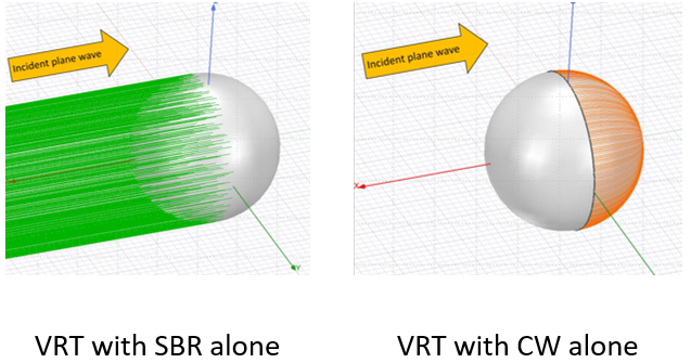
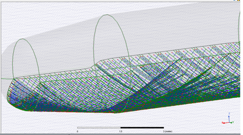
This feature includes a Visual Ray Trace (VRT) capability, which allows you to visualize creeping rays before running the simulation. The VRT is an essential tool for tuning CW parameters and diagnosing problems. The figure shows a VRT performed in the AEDT GUI. The CW rays travel along the surface starting from the shadow boundary, which divides the regions that are directly visible and shadowed with respect to the direction of incidence of the plane wave. Users are strongly encouraged to perform a VRT before running the simulation to help ensure the rays are propagating as expected

A VRT example is show below, first with SBR rays alone and then with plane wave CW rays alone.

When you use the Creeping Wave feature, before you simulate the design, you must set parameters in the Hybrid Regions and in the Solution Setup. After running a simulation, you can create RCS reports and create field plots of creeping rays.

Prerequisites

Create an HFSS design with SBR+ regions, either driven model or terminal solution type or SBR+ solution type.

Create a plane wave source for an RCS simulation with an SBR+ Region.

Process Flow for Setting up and Simulating an SBR+ Design for Creeping Waves for RCS

1. Create an HFSS design with SBR+ region (either driven modal solution type or SBR+ solution type).
2. Add geometries.

These can be either light weight geometries, or conventional Modeler geometries.

You can specify how SBR+ curvature extraction is to be handled per geometry component/part. By default, the curvature extraction is applied on all SBR+ faces in the design. You can disable curvature extraction on selected faceted faces or objects by using this mesh operation.

When object curvature information is available in the original geometry, the Apply Curvilinear Elements option may be used. This option avoids the curvature extraction approximation by passing curvature information directly to the SBR+ solver, which is more accurate.

3. Add an Incident Plane Wave source.
4. Add a Solution setup and in the SBR+ Solution Setup, Options tab or or HFSS with Hybrid and Arrays driven modal solution setup Hybrid tab select Enable Creeping Wave. (Note that this option is only available in the solution setup dialog if a near-field link to an HFSS source such as a FEBI or IE region excitation/boundary is present in the design.)
   

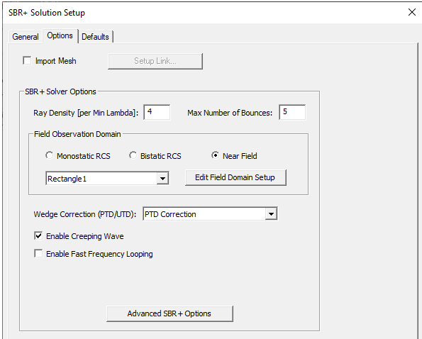
Select Advanced SBR+ Options and in the SBR+ Advanced Options dialog check Customize Creeping Wave Options to enable the Creeping Wave tab..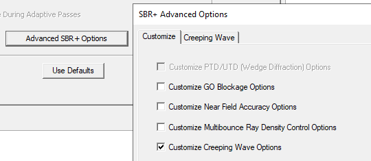

Select the Creeping Wave tab to set parameters.

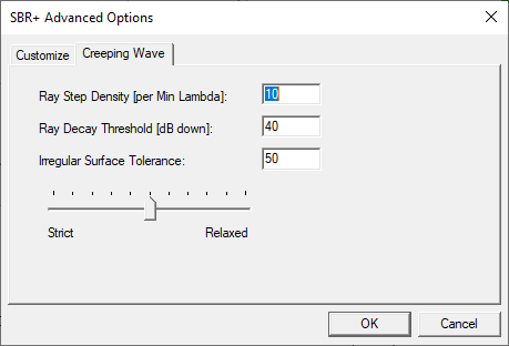
Ray Step Density controls the longitudinal sampling along the direction of propagation. The lateral sampling is determined by the SBR ray density.

Ray Decay Threshold controls how far the creeping rays propagate by terminating each ray once its power density decay (defined as dB down from its level at its starting point at the shadow boundary) exceeds this threshold.

Irregular Surface Tolerance is a single control for a collection of tolerances that determine creeping rays’ sensitivities to local surface irregularities that theoretically should block their further propagation. Moving the slider toward Relaxed allows creeping rays to propagate through small surface irregularities that may arise through defects in the input geometry or due to limitations of curvature extraction accuracy. However, setting this tolerance too relaxed may allow creeping waves to pass through concave surfaces, saddle surfaces, or wedges, which are not supported by creeping wave physics. Therefore, you are strongly encouraged to perform a creeping-wave visual ray trace (VRT) to determine an acceptable setting for this tolerance, which will differ from model to model. The intention is that creeping rays only propagate over the convex portions of surfaces, and some user judgment is required in correctly setting the Irregular Surface Tolerance for each situation.

5. Run simulation.

You should see the progress bar reporting both SBR and Creeping Wave ray shoots during the EMA3D solver part of the run.

6. Generate RCS plots

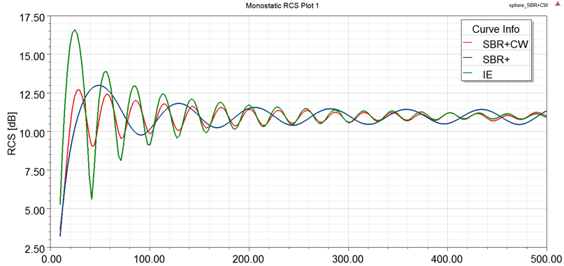
Right click on Result and select Create Monostatic RCS Report > Rectangular Plot. For the Report window, select Monostatic RCS as the Category, MonostaticRCSTotal as the Quantity, with dB as the Function, and click New Report.

A comparison of RCS solved by various methods for a 1-meter radius sphere is shown below. Comparing with the reference integral equation (IE) solution, and also the exact Mie series solution (not shown), the SBR+ solution with creeping wave (SBR+CW) better captures the oscillatory behavior of RCS over the simulation frequency band. For a sphere illuminated by a plane wave, the “shadow boundary” is the great circle perpendicular to the incident wave direction. The slower oscillation versus frequency predicted by SBR+ alone is caused by the wave interference of the back-scattered direct return from the leading surface of the sphere with a false diffraction from the shadow boundary where physical optics (PO) currents abruptly (and non-physically) terminate. Instead, currents should smoothly weaken when crossing from the lit half to the shadowed half of the sphere. The faster (and correct) oscillation of the IE and SBR+CW solutions is caused by the wave interference of the direct return with the delayed return of a creeping wave passing around the back of the sphere and coming out toward the front again. Since the difference in path length between these two scattering mechanisms (direct and around-the-back) is larger than the difference in that of the former (direct and false shadow boundary diffraction), the beat frequency of the interference is higher.