
Setting Up Adaptive Single-Objective (Gradient) Optimizer
Following is the procedure for setting up an optimization analysis using the Adaptive Single-Objective (OSF + Kriging + MISQP) Optimizer. Once you have created a setup, you can Copy and Paste it, and then make changes to the copy, rather than redoing the whole process for minor changes.
This gradient-based method employs automatic intelligent refinement to provide the global optima. It requires a minimum number of design points to build the Kriging response surface, but, in general, this method reduces the number of design points necessary for the optimization. Failed design points are treated as inequality constraints, making it fault-tolerant.
The Adaptive Single-Objective method is available for input parameters that are continuous, including those with manufacturable values. It can handle only one output parameter goal, although other output parameters can be defined as constraints. It does not support the use of parameter relationships in the optimization domain. For more information, see Adaptive Single-Objective Optimization (ASO). It requires advanced options. Ensure that the Show Advanced Options check box is selected.
-
Set up the variables you want to optimize in the Design Properties dialog box. The variables must be swept in a Parametric setup.
-
Click
- Under the Goals tab, choose the optimizer by selecting Adaptive Single Objective (Gradient) from the Optimizer drop-down menu.
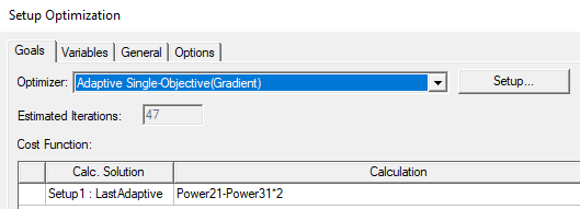
- Optionally press the Setup button to open the Optimizer Options window and check Advanced Options.
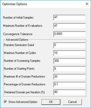
- Number of Initial Samples: Number of samples generated for the initial Kriging and after all domain reductions for the construction of the next Kriging. You can enter a minimum of (NbInp+1)*(NbInp+2)/2 (also the minimum number of OSF samples required for the Kriging construction) or a maximum of 10,000. The default is (NbInp+1)*(NbInp+2)/2.
Because of the Adaptive Single-Objective workflow (in which a new OSF sample set is generated after each domain reduction), increasing the number of OSF samples does not necessarily improve the quality of the results and significantly increases the number of evaluations
- Maximum Number of Evaluations:Stop criterion. Maximum number of evaluations (design points) that the algorithm is to calculate. If convergence occurs before this number is reached, evaluations stop. This value also provides an idea of the maximum possible time it takes to run the optimization. The default is 20*(NbInp +1).
- Convergence Tolerance: Stop criterion. Minimum allowable gap between the values of two successive candidates. If the difference between two successive candidates is smaller than the value for Convergence Tolerance multiplied by the maximum variation of the parameter, the algorithm is stopped. A smaller value indicates more convergence iterations and a more accurate (but slower) solution. A larger value indicates fewer convergence iterations and a less accurate (but faster) solution. The default is 1E-06.
- Random Generator Seed: The value for initializing the random number generator invoked internally by OSF. The value must be a positive integer. This property allows you to generate different samplings by changing the value or to regenerate the same sampling by keeping the same value. The default is 0.
- Maximum Number of Cycles: Number of optimization loops that the algorithm needs, which in turns determines the discrepancy of the OSF. The optimization is essentially combinatorial, so a large number of cycles slows down the process. However, this makes the discrepancy of the OSF smaller. The value must be greater than 0. For practical purposes, 10 cycles is usually good for up to 20 variables. The default is 10.
- Number of Screening Samples: Number of samples for the screening generation on the current Kriging. This value is used to create the next Kriging (based on error prediction) and verified candidates.
You can enter a minimum of (NbInp+1)*(NbInp+2)/2 (also the minimum number of OSF samples required for the Kriging construction) or a maximum of 10,000. The default is 100*NbInp for a Direct Optimization system. There is no default for a Response Surface Optimization system.
The larger the screening sample set, the better the chances of finding good verified points. However, too many points can result in a divergence of the Kriging.
- Number of Starting Points: Determines the number of local optima to explore. The larger the number of starting points, the more local optima explored. In the case of a linear surface, for example, it is not necessary to use many points. This value must be less than the value for Number of Screening Samples because these samples are selected in this sample. The default is the value for Number of Initial Samples.
- Maximum Number of Domain Reductions: Stop criterion. Maximum number of domain reductions for input variation. (No information is known about the size of the reduction beforehand.) The default is 20.
- Percentage of Domain Reductions: Stop criterion. Minimum size of the current domain according to the initial domain. For example, with one input ranging between 0 and 100, the domain size is equal to 100. The percentage of domain reduction is 1%, so the current working domain size cannot be less than 1 (such as an input ranging between 5 and 6). The default is 0.1.
- Retained Domain per Iteration (%): Advanced option that allows you to specify the minimum percentage of the domain you want to keep after a domain reduction. The percentage value must be between 10 and 90. A larger value indicates less domain reduction, which implies better exploration but a slower solution. A smaller value indicates a faster and more accurate solution, with the risk of it being a local one. The default percentage value is 40.
- Number of Initial Samples: Number of samples generated for the initial Kriging and after all domain reductions for the construction of the next Kriging. You can enter a minimum of (NbInp+1)*(NbInp+2)/2 (also the minimum number of OSF samples required for the Kriging construction) or a maximum of 10,000. The default is (NbInp+1)*(NbInp+2)/2.
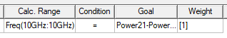
- Add
a cost function by selecting the Setup Calculations
button to open the Add/Edit Calculation dialog box.
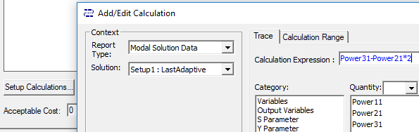
When you have created the calculation, click Add Calculation to add it to the Optimization setup, and Done to close the Add/EditCalculation dialog box.
- In the Optimization setup, in the Goal column drop-down menu, select either Edit as Expression... or Edit as Numeric Value....
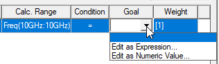
- This reopens the Add/Edit Calculation dialog box. If you are satisfied with the expression or value displayed, click Done to close the dialog box. This enters the expression/value into the Goal column.
- In the Optimization setup, if you want to select a Cost Function Norm Type:
- Check the Show Advanced Option check box.
The Cost Function Norm Type pull-down list appears.
- Select L1, L2, or Maximum.
A norm is a function that assigns a positive value to the cost function.
For L1 norm the actual cost function uses the sum of absolute weighted values of the individual goal errors. For L2 norm (the default) the actual cost function uses the weighted sum of squared values of the individual goal error. For the Maximum norm the cost function uses the maximum among all the weighted goal errors, which means that it is always less than zero. (For further details, see Explanation of the L1, L2, and Max Norms in Optimization.)
The norm type doesn't impact goal setting that use as condition the "minimize" or "maximize" scenarios.
- Check the Show Advanced Option check box.
- Optionally, set the Acceptable Cost and Cost Function Noise.
- Optionally, click the button for setting HPC and Analysis Options, which allows you to select or create an analysis configuration.
- In the Variables tab, specify the
Min/Max values for variables included in the optimization.
- You may also override the variable starting values by clicking the Override check box and entering the desired value in the Starting Value field.
- Optionally, modify the values of fixed variables that are not being optimized.
- Optionally, set Linear constraints.
- Select the View all columns check box to see all columns, including hidden columns.
- In the General tab, specify whether
Optimetrics should use the results of a previous Parametric analysis
or perform one as part of the optimization process.
Enabling the Update design parameters' value after optimization check box will cause Optimetrics to modify the variable values in the nominal design to match the final values from the optimization analysis.
- Under the Options tab, if you want to save
the field solution data for every solved design variations in the optimization
analysis, select Save Fields And Mesh.
Note:
Do not select this option when requesting a large number of iterations as the data generated will be very large and the system may become slow due to the large I/O requirements.
You may also select Copy geometrically equivalent meshes to reuse the mesh when geometry changes are not required, for example when optimizing on a material property or source excitation. This will provide some speed improvement in the overall optimization process.