
Assigning SBR+ Hybrid Regions
HFSS can use shooting and bouncing ray (SBR) technology to compute the scattered field contribution of defined platform geometry via one-way coupling. This allows you to efficiently calculate installed near field patterns, far-field patterns and coupling (S-parameters) between antennas in the presence of an electrically large scattering geometry.
Note that the same SBR+ mesh used for both SBR+ simulation and VRT is also used in extracting wedges according to the user-specified criteria. This is done so that the wedge locations extracted are very near the physical edges of the SBR+ geometry model in the simulation, preserving accuracy of the line-of-sight visibility check for wedges.
- An SBR+ Region can only be assigned to no-solve inside object (metal).
- When an object is assigned as an SBR+ region, Boundary conditions (BCs) may be assigned to the geometry inside the SBR+ region(s), but there are some limitations in what boundary conditions are supported. HFSS currently supports assignment of Perfect E, Perfect H, Impedance, Finite Conductivity, and Layered Impedance boundaries to geometry in the SBR+ region. Other boundaries are not yet supported for SBR+, and produce an error. Infinite Ground Planes are not supported with SBR+. Note also that surface roughness must be set to “0” for all BCs assigned to SBR+ region geometry.
- An SBR+ Region cannot be contained by a dielectric cavity.
- Incident plane waves are allowed. If you include an incident plane wave in the design, the Hybrid tab for the Driven Solution Setup dialog includes options for RCS type as Monostatic or Bistatic.
- If an SBR+ Region is assigned, the design becomes one way coupled. (See Assigning Hybrid Regions.) You can use the Set SBR+ Source Regions command to group source regions for SBR+ for two-way couplings between the grouped regions.
- Terminal ports with multiple terminals are supported if a an SBR+ region is present.
- Designs with SBR+ regions provide options to view total, scattered, or incident fields.
- SBR+ Region simulations can benefit from GPU Acceleration. See Setting HPC and Analysis Options.
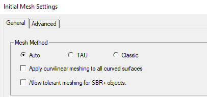
- If your design contains an SBR+ Hybrid Region, you have an option on the Initial Mesh Settings dialog to Allow tolerant meshing for SBR+ regions, which can speed up the solve.
- If you want to consider far fields or near fields, the field sample points for SBR+ Hybrid regions must be defined as part of the simulation setup, rather than during post processing as is done for HFSS near and far fields. See the discussion of the Setup dialog box, Hybrid tab in step 3 below.
- HFSS with Hybrid and Arrays designs that include blockages have an enhanced work flow described.
-
When a project contains SBR+ region and the following error appears: "[error] Solving adaptive frequency ... (Domain solver), process hf3d error: Error in using SBR+ region: Each source region should contain at least one excitation."
"Each source region should contain at least one excitation" means there is at least one source region without an excitation. To work around the issue, please go to Set SBR+ Source Regions and, select all regions and click "Group".
You must select an appropriate object in order to enable the menu.
To assign an SBR+ Hybrid Region:
- Select the object you want to assign as an SBR+ Region, and use one of the following menus:
HFSS > Hybrid > Assign Hybrid > SBR+ Region
Right-click in the Modeler window and select Assign Hybrid > SBR+ Region.
Select the Hybrid Regions icon in the Project
tree, right-click, and click Assign > SBR+ Region.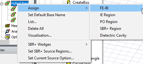
The dialog for Hybrid
Region opens, showing the default name and type selection
as IE Region. Because you may decide to change an assignment for IE Regions,
and PO Regions, the dialog shows these types as radio button selections.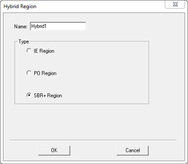
- When you OK the dialog box, the assignment appears in the Project Tree under Hybrid Regions.
- SBR+ Solver Options are enabled in Solve setups for HFSS when an SBR+ Region is present.
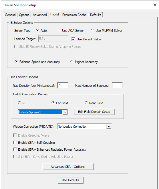
You can set Ray Density Per Wavelength and Maximum Number of Bounces, and if you have not done so, create or edit an infinite sphere setup for Far Field Observation. See Setting Hybrid Region Parameters for HFSS. You can also choose to Skip SBR+ Solve During Adaptive Passes. SBR+ regions are not being mesh adapted and SBR+ solutions have no impact on field solutions on FEM or IE regions. However, SBR+ does impact stopping criteria in some cases such as coupling between two separate source antennas. Therefore, to speed up mesh adaption, you can choose to not solve SBR+ regions until source regions have converged in isolation. However, SBR+ does impact stopping criteria in some cases in the form of cache expression such as coupling between two separate source antennas or far field pattern. In such cases, SBR+ solve could not be skipped. Moreover, SBR+ solve is always launched when the maximum number of passes is reached regardless of source region convergence.
If you created an Incident Plane Wave for the design, the Hybrid tab lets you make an RCS Type selection for Monostatic or Bistatic.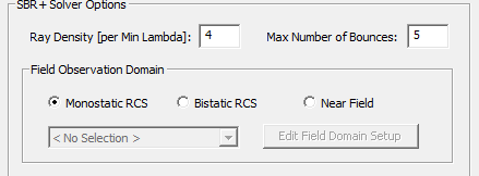
If you select Monostatic, the infinite sphere setup is disabled. In this case, the solver computes the scattered field in the direction of the plane wave. The Reporter will not require a geometry selection, and offers a range of Monostatic quantities for Monostatic RCS traces. See Generating Reports for Monostatic RCS.
If you select have assigned both an SBR+ region and an Incident Plane wave, and select Bistatic as the RCS Type, the Near Field and Far Field Observation domain fields are enabled, and the Far Field Radiation Sphere Setup dialog appears as follows, allowing you to create an infinite sphere for a Far Field or a rectangle for examining near fields. You can edit an existing Far Field Infinite Sphere or Near Field Rectangle setup by selecting from the drop down menu and clicking Edit Field Domain Setup.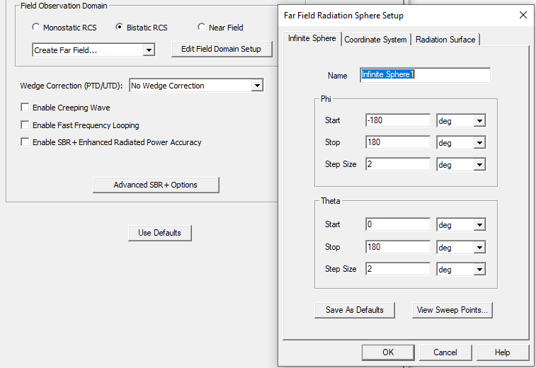
If you have created one or more field observation domains, these are listed on the dropdown. You can edit an existing Far Field Infinite Sphere or Near Field Rectangle by clicking Edit Field Domain Setup.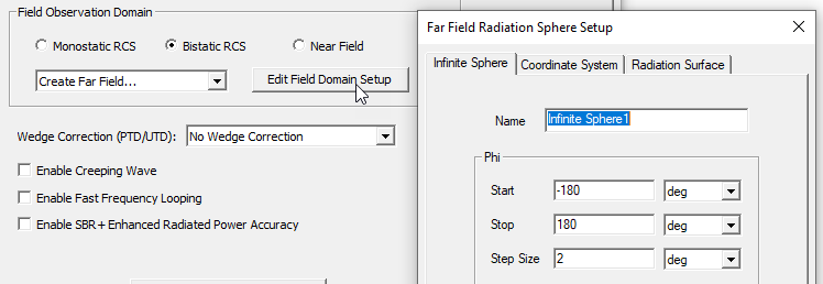
For Near Field rectangle setups, you can use the feature described in Overlay Contour Plot of Near Field on Rectangle. - Enable SBR+ Self Coupling computation capability for driven designs means that the diagonal S-param term takes into consideration the SBR+ scattering effect, and is more accurate. For a discussion of SBR coupling see, Select Tx/Rx Antennas for SBR+ Solutions.

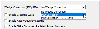
- The PTD/UTD Simulation Settings allow for the inclusion of additional wedge diffraction phenomenology that can improve the accuracy of SBR+ simulations. You can opt out of using the PTD/UTD settings, or select PTD Correction or PTD Correction + UTD Rays. Selecting one of the PTD Correction options enables a field for specifying PTD Edge Density. This controls how densely wedges are segmented when establishing line of sight from the field source (for example, Tx antenna) to each wedge segment.
For SBR+ simulations, the Physical Theory of Diffraction (PTD) and Uniform Theory of Diffraction (UTD) features can account for additional phenomenology not well predicted by plain SBR due to truncation of uniform Physical Optics (PO) currents at sharp angular discontinuities (“wedges”) on metallic surfaces and blockage of SBR’s Geometrical Optics (GO) rays. PTD is a numeric correction to the scattered fields radiated by PO currents near wedges. UTD launches bundles of edge-diffraction rays from directly illuminated portions of each wedge along the Keller cone. Once launched, the UTD rays behave exactly like regular SBR rays, propagating according to GO and painting PO currents at each bounce that contribute to the scattered field. The UTD rays often illuminate portions of the SBR scattering geometry that are never reached by SBR GO rays launched directly from the field source.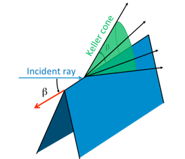
The PTD and UTD wedge features are only deployed for metallic wedges with line-of-sight visibility from the source (Tx) location. If either adjacent surface of the wedge is non-PEC and not within the tolerance for PEC-like, or if the entire edge segment is not visible to the source, the wedge will be ignored in the SBR+ simulation and for visual ray tracing (VRT).
- Advanced Option for NF Accuracy Settings for SBR+
The NF Accuracy settings (Beta feature, NF Accuracy Controls for SBR+) provide access to methodology settings relating to cases where Tx antennas, Rx antennas, and near-field observation points are in proximity to the scattering geometry (i.e., the platform CAD model). When this feature is switched off, HFSS SBR+ uses default near-field accuracy settings that should be adequate for most situations, including close-proximity Tx/observer conditions that this feature is designed to tune.
- Advanced Option for Multibounce Ray Density
By option you can select the Advanced SBR+ Options and enable Customize Multibounce Ray Density Control Options.
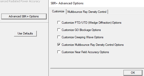
You can then select the Multibounce Ray Density Control tab.
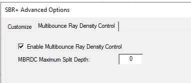
Use the checkbox to Enable Multibounce ray density and enter the maximum number of subdivisions to be used in the solve. Enabling the feature may increase the solve time.
The MBRDC Maximum Split Depth field value increases the number of spawned ray tracks on each ray bounce. The MBRDC algorithm is designed to achieve the ray density per wavelength criterion at any bounce depth. If a footprint at depth N in a ray track does not satisfy the ray-density criterion, the MBRDC algorithm attempts a refined ray shoot from an earlier bounce, just for the ray in question. The size of the triggering footprint informs the level of refinement. If the refined shoot is not successful in achieving the desired footprint size, or new footprints are too large, the MBRDC algorithm attempts further, recursive refinements. The MBRDC Maximum Split Depth setting limits how aggressively the refinement algorithm is applied by specifying the maximum number of split recursions. For this reason, linear increases in Maximum Split Depth can yield a geometric progression in the total number of rays shot and associated solution time.
When both MBRDC and UTD are enabled, first-bounce UTD rays and bright points on wedges are recomputed during the MBRDC splitting process, but only the original raytrack is rendered up to the 1st bounce. Similarly, length-based ray filters are applied to the original UTD initial ray track up to 1st bounce rather than using the information in the additional MBRDC tracks. This is a known limitation.
- Advanced Option for Geometrical Optics (GO) Blockage
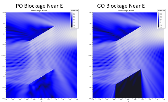
SBR+ normally applies a physical optics (PO) blockage model where blockage effects emerge from partial cancellation of the incident field by the scattered field. PO blockage not only occurs in connection with the incident field from the Tx antennas, but also within the scattered field itself when reflected fields from the previous bounce are diminished by a blocking surface along the geometrical-optics (GO) reflection path at the current bounce by evaluating the scattering contribution of the incident ray field at that bounce.
In cases of significant blockage by a large obstruction, the PO blockage model requires accurate currents over the extent of the obstruction. Sometimes, this is hard to achieve in the ray tracing approximation. For example, the obstruction may not be well illuminated by direct rays from the Tx antenna or multi-bounce rays after an earlier reflection. An alternative is to use a GO blockage model where scattered field contributions are added to an observation point subject to a line-of-sight (LOS) blockage check performed by the ray tracer. In some cases, this is more accurate than the default PO blockage formulation, while in others it is less accurate. GO blockage also entails a non-trivial computational cost, as the blockage check with the ray tracer must be performed for each observation angle (or point) for each ray hit point.
In addition to GO Blockage for SBR and UTD ray tracks, this feature is also available for PTD and CW.
Limitations for GO Blockage:
GO Blockage formulation is suited specifically for SBR+ ray tracks, including UTD ray tracks. While GO Blockage for CW and PTD has been implemented for the first time in this release, results can be surprising and/or inaccurate, as a limitation of the methodology.
Summary Workflow for GO Blockage:
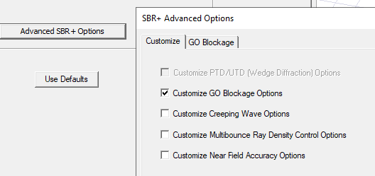
Click the Advanced SBR+ Options button to open the SBR+ Advanced Options window. On the Enable tab, Check GO Blockage Options to enable the GO Blockage tab.
On the GO Blockage tab, you have check box options to enable or disable GO Blockage, Surface self-block, and GO Blockage Checks for Incident Fields..
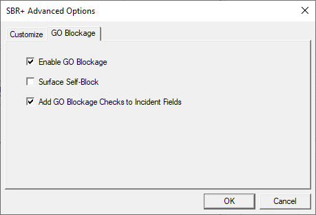
Surface Self-Block: if enabled, the surface where the footprint is radiated from is used for blockage check, that is, anything below the surface with respect to the incoming ray is not in line of sight. If the setting is disabled, the footprint surface is not used for blockage checks (anything below the surface with respect to the incoming ray is in line of sight), but other surfaces are used for blockage.
For example, consider a parametric beam antenna illuminating a series of plates.
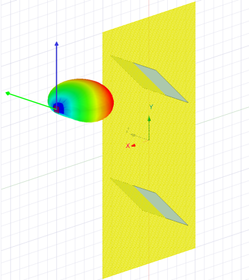
In the plots, the shadows behind the plates are much more pronounced with GO Blockage enabled, but the fields have non-physical discontinuities.
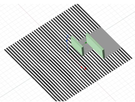
Add GO Blockage Checks to Incident Fields: if enabled, GO blockage effects will also be calculated for the incident field via line-of-sight checks from sources to field points, effectively computing a direct field in the Geometrical Optics sense. For example, the figure below shows the total E-field of a planewave incident on PEC bodies with this option enabled.
- Wedge settings for the SBR+ simulation with PTD/UTD are only accessible for an SBR+ design. Wedges are based on theAutomatic Wedge Generation settings, optional Interactive Wedge Editing, and the initial mesh. The initial mesh is automatically generated on launch of the SBR+ Wedge Settings dialog box, if needed. The dialog will not launch if an initial mesh is not available and cannot be generated. The SBR+ Wedges submenu can be accessed through a right-click the Hybrid Regions icon in the Project tree.
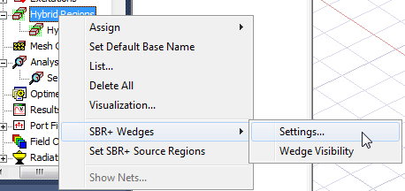
The submenu contains the option for opening the SBR+ Wedge > Settings dialog box and a checkable option for enabling or disabling Wedge Visibility. If visible, wedges are shown as thick red lines in 3D model window for automatically generated wedges, and as blue lines for interactively edited wedges. Visualization is turned off when there is design edits that invalidate the initial mesh.
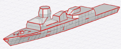
The SBR+ Wedge Settings dialog box contains the Automatic Wedge Generation parameters and the Interactive Wedge Editing feature.
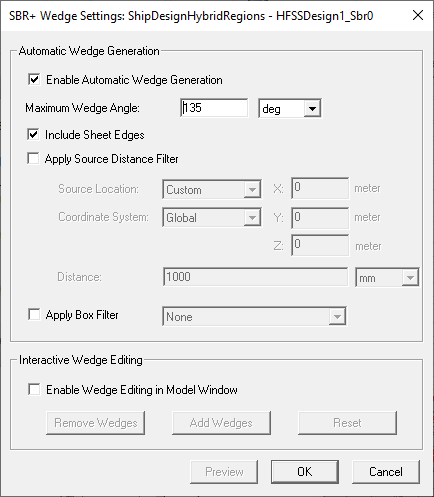
The Wedge Generation parameters are used to determine the candidate set of wedges to be included, with optional filters that can restrict their location on the geometry. The final set of wedges to be used in the SBR+ simulation is the intersection of all the wedge generation criteria, and the effects of any optional Interactive Wedge Editing. complete flexibility in specifying where the wedges are to be used for the simulation. This is important since adding many wedges on very large geometry structures (aircraft, vehicles, etc.) can significantly impact the SBR+ simulation time.
Enable Automatic Wedge Generation.
By default, the checkbox is enabled, allowing access to the automatic features and parameters. If you un-check it, the automatic features are disabled. You can independently enable Wedge Editing.
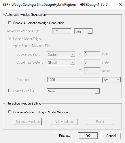
Wedges added through Automatic Wedge Generation are displayed in red.
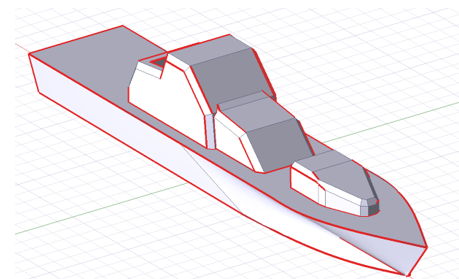
Maximum Wedge Angle:
An angular criteria can be specified for the maximum wedge angle to help filter the desired set of wedges - default value is 135 deg. This wedge angle ranges from minimum 0 deg to maximum 180 deg. All wedges are included that are less than or equal to the specified maximum angle. An angle equal to 0 deg would be created by a “collapsed” wedge (like a closed hinge), while an angle equal to 180 deg would be created by a completely “open” wedge (like a fully open hinge). You can assign a design variable to Maximum Wedge angle, but you cannot create a design variable within the dialog.
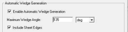
Include Sheet Edges:
You can choose to include or exclude the edges from sheets (non-connected edges, also known as “knife edges”). The default value is true which includes these edges. Sheet edges are triangle edges with no adjacent/connected triangle along that edge. In the physical object we are modeling these may represent extremely thin surfaces such as metal “fins”, etc.
Optional parameters:
Apply Source Distance filter:
A “source distance filter” allows you to specify that you want to include wedges within a finite 3D distance from a point (the “source”).
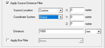
You can choose model Points from drop down as source location, or specify the absolute X, Y, Z in model units. X, Y, Z can be specified in global coords or relative to a custom CS. When you select a geometry Point, its coordinate system and X, Y, Z are displayed.
The Distance default is 1 <model unit>. You can assign an existing design variable to the Distance. Default value is false (no Source Distance Filter).
Apply Box Filter:
You can select any non-model box that is aligned with the Global Coordinate System axes via a drop-down menu, within which wedges will be included. Default value is false (no Box Filter).
Optional Interactive Wedge Editing
This feature provides complete flexibility in specifying where the wedges are to be used for the simulation. This is important since adding many wedges on very large geometry structures (aircraft, vehicles, etc.) can significantly impact the SBR+ simulation time.
Checking the Enable Wedge Editing the Model Window box enables the buttons for removing wedges from selected geometries (faces, objects, etc.) , adding wedges to selected geometries, and resetting edits.
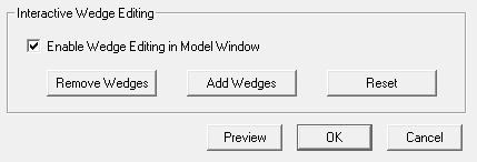
After you select a geometry and Add Wedges, the interactively added wedges appear in blue.
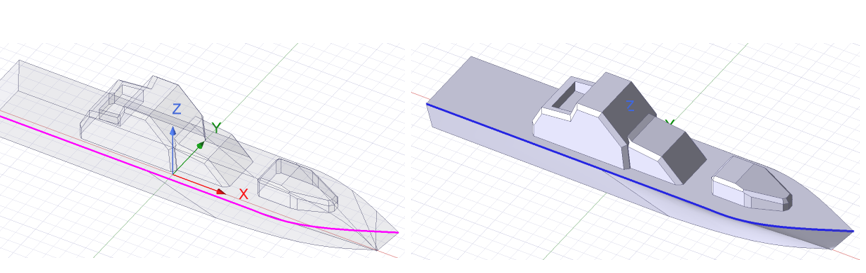
If you select Remove Wedges, all wedges on the selected geometry objects are removed. These can be automatically generated wedges or interactively added wedges.
Click Reset Wedges to undo all interactive wedge editing operations. A confirmation dialog appears. Press Yes to reset all wedge editing operations. The reset button is disabled if no wedge edit operations are present.
Current Limitations on PTD/UTD Wedge Generation/Editing
Situations where wedges cannot be generated:
Light Weight Imported STL Geometries: STL models imported as light weight geometries are currently not supported for interactive wedge editing (as of R24.1).
In the Initial Mesh Settings for SBR+ Solution type or for HFSS with Hybrid and Arrays that include SBR+ regions, you can turn off tolerant meshing.
In this case you should consider Current Limitations on PTD/UDT Wedge/Generation Editing.
Configure Simulation with SBR+ Antenna Geometry Blockage (HFSS with Hybrid and Array Solution Type):
The typical configuration begins with a fully integrated model with all geometry. You then select the near antenna region including any nearby geometry interacting with the antenna for analysis by HFSS – either by identifying these objects by hybrid region assignment, or by copying them out to a separate source antenna design to be solved with the HFSS solver, etc. The nearby antenna geometry could even be something different than what is used for the integrated model, such as a flat plate or other structure for considering the nearby antenna interactions. This source antenna design should likely be enclosed in a FE-BI region to allow for easier downstream processing, whether we are in a Hybrid or SBR+ solution type. If you use a separate source antenna design, you can re-introduce it to the target design with the full geometry model by creating a 3D component for an antenna that is a linked design to the source design. This means you no longer need to designate any “Model Blockage” when setting up the linked design. You do this as a separate step outside creation of the linked design by selecting geometry from the SBR+ region to be designated as “Model Blockage” associated with a particular source antenna. Note there is no restriction on what objects and/or materials can be designated as “model blockage” geometry. Also note that for either solution type, SBR+ or hybrid HFSS-SBR+, that this selection will be from the available SBR+ region geometry objects, which is different than the previous workflow. Once you select these antenna blockage geometries for each source antenna, HFSS with SBR+ can solve the combined target SBR+ design.
You can also specify HFSS Hybrid solution type with SBR as a source for a target SBR+ design as a far field linked design with antenna blockage support. In such cases, you can optionally configure antenna blockage settings in the source design. You must solve the design before you can link it to the SBR+ target design. You cannot link a Hybrid solution type with with SBR+ regions source design to a target HFSS design.
The preferred work flow is this.
- Create/open an design with HFSS with Hybrid and Arrays solution type.
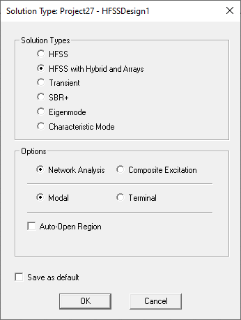
- Configure the source excitation, including adding or creating any nearby geometry.
- Create a hybrid FE-BI region to enclose the source excitation and all the nearby geometry objects to be part of the HFSS simulation.
- Add all the additional geometry objects that will be part of the hybrid analysis, configuring all materials/boundaries as desired.
- Create/assign a hybrid SBR+ region to all the desired geometry objects to the design.
- If you want to designate multiple SBR+ geometry objects as blockage, select them in the 3D Modeler window and create an object selection using Modeler > Named Selection > Create > Object Selection. You may want to name the selection appropriately. If only a single object is to be designated as a geometry blockage, skip this step.
- Open the dialog to configure SBR+ source regions (which includes antenna blockage) via the menu option for Hybrid Regions > Set SBR+ Source Regions....
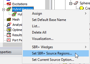
This opens the Set SBR+ Source Regions dialog box: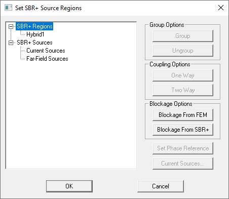
Click the Blockage from SBR+ button to bring up the antenna blockage dialog box: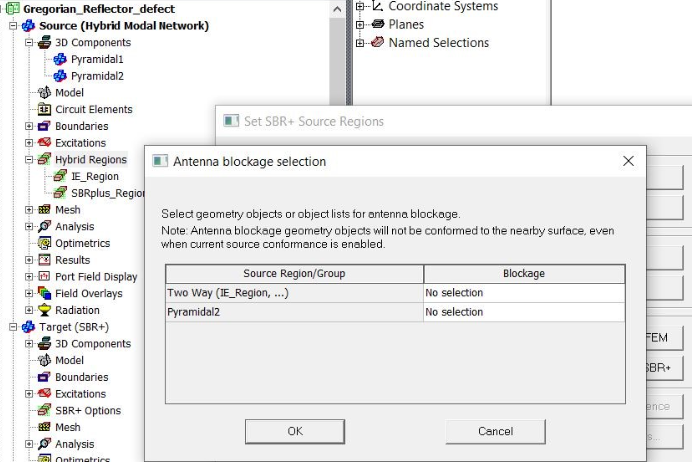
- (Optional) Configure antenna blockage settings in the source design. Both blockage dialogs (FEM and SBR+) can be used concurrently.
For each antenna source, use the “Blockage" column to select the geometry blockage from the drop-down. Each cell in the column contains a drop-down list of all geometry objects and all user-created object selections.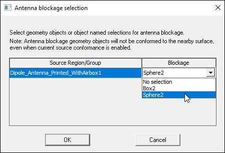
- Click OK to save the configuration.
- Create an Analysis Setup.
- Run the simulation.
- For Hybrid Solution type with SBR+ as a source for an HFSS SBR+ design (the target design), create an antenna link to the source design. Only far field links are currently supported. Source designs with multiple FEBI regions and blockage selections are not supported.
-
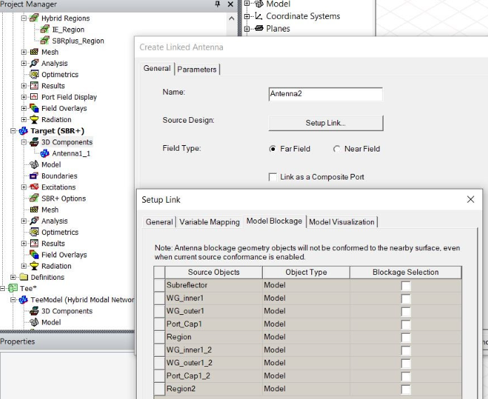
(Optional) Configure antenna blockage settings in the link dialog. SBR+ region objects from the source design should appear in the object list. Objects selected for blockage in the source design will be selected in the link blockage dialog by default.
-
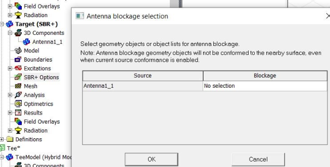
(Optional) Configure antenna blockage settings in the target design antenna blockage dialog. These selections will work together with the link dialog blockage selections.
- Analyze target design and inspect results. The incident field shown in the target design should match the total field of the source design.
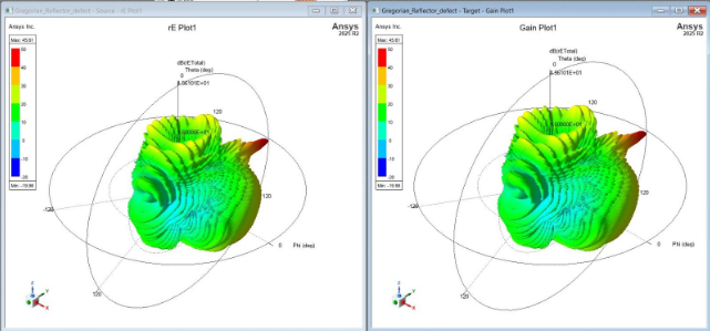
Only object selections that contain exclusively SBR+ can be selected for antenna blockage.