


The following topics are discussed in this section:
PSD analysis is performed with a large number of modes first.
Reduction of the number of modes used also reduces the solution time, but at the expense of accuracy. Accuracy can be improved without a significant increase in the solution time by using residual vectors.
The figure below shows the elapsed and CPU times with and without the residual vector method and the expansion of the modes. A significant reduction in the solution time is achieved by storing the modal element results.
Figure 20.11: Solution Times With and Without Store Modal
Results (MSUPkey = YES on the
MXPAND command)
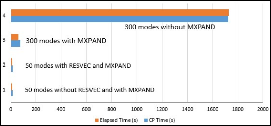
The solution time is slightly increased with the residual vector. For 50 modes, the elapsed time with and without the residual vector is 12 seconds for both.
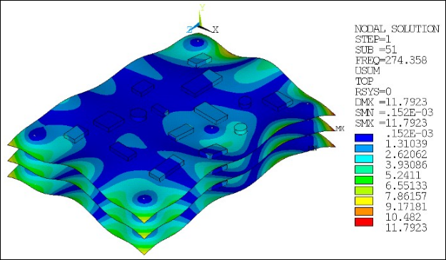
The mode shape of the residual vector obtained using 50 modes (the 51st mode being the residual vector) is shown in the figure below. These results were obtained using a post processing command snippet (shown below) since they are not supported in Workbench Mechanical. Note that the residual vector corresponds to a displacement in the y direction.
/POST1
/show,png
/view,1,1,1,1
set,1,51                         ! Define set to be read from 51st subset of first set
PLNSOL,u,sum,,,,avg              ! Plot vector sum of nodal displacement as continuous contours
*get,freq_mode51,MODE,51,freq    ! Get frequency corresponds to residual vector mode shape
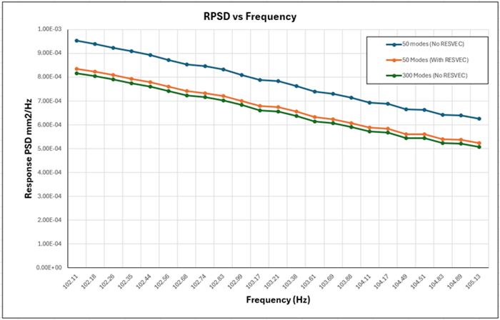
The residual vector method uses an additional vector computed in the modal analysis pass in addition to the eigenvectors in the modal transformation. This increases the accuracy of the response solution. RPSD displacement solutions with and without the residual vector are listed in the table below. For 50 modes without the residual vector, accuracy of the results is poor, as shown in column A in the following table. Accuracy is significantly improved with the use of the residual vector, as shown in column B.
| Number of Modes | %
Difference with Column C | ||||
| Frequency | 50
(No RESVEC) Column A | 50
(With RESVEC) Column B | 300
(Full Model) Column C | 50 (No RESVEC) | 50 (With RESVEC) |
| 102.11 | 9.5232 x 10⁻⁴ | 8.3521 x 10⁻⁴ | 8.1689 x 10⁻⁴ | 16.58 | 2.24 |
| 102.18 | 9.3896 x 10⁻⁴ | 8.2284 x 10⁻⁴ | 8.0425 x 10⁻⁴ | 16.75 | 2.31 |
| 102.26 | 9.2416 x 10⁻⁴ | 8.0873 x 10⁻⁴ | 7.9024 x 10⁻⁴ | 16.95 | 2.34 |
| 102.35 | 9.0811 x 10⁻⁴ | 7.9308 x 10⁻⁴ | 7.7504 x 10⁻⁴ | 17.17 | 2.33 |
| 102.44 | 8.9266 x 10⁻⁴ | 7.7836 x 10⁻⁴ | 7.6042 x 10⁻⁴ | 17.39 | 2.36 |
| 102.56 | 8.7298 x 10⁻⁴ | 7.5960 x 10⁻⁴ | 7.4179 x 10⁻⁴ | 17.69 | 2.40 |
| 102.68 | 8.543 x 10⁻⁴ | 7.4180 x 10⁻⁴ | 7.2411 x 10⁻⁴ | 17.98 | 2.44 |
| 102.74 | 8.4532 x 10⁻⁴ | 7.3324 x 10⁻⁴ | 7.1562 x 10⁻⁴ | 18.12 | 2.46 |
| 102.83 | 8.3229 x 10⁻⁴ | 7.2083 x 10⁻⁴ | 7.0329 x 10⁻⁴ | 18.34 | 2.49 |
| 102.99 | 8.1037 x 10⁻⁴ | 6.9995 x 10⁻⁴ | 6.8255 x 10⁻⁴ | 18.73 | 2.55 |
| 103.17 | 7.875 x 10⁻⁴ | 6.7817 x 10⁻⁴ | 6.6091 x 10⁻⁴ | 19.15 | 2.61 |
| 103.21 | 7.8266 x 10⁻⁴ | 6.7356 x 10⁻⁴ | 6.5634 x 10⁻⁴ | 19.25 | 2.62 |
| 103.38 | 7.6302 x 10⁻⁴ | 6.5486 x 10⁻⁴ | 6.3777 x 10⁻⁴ | 19.64 | 2.68 |
| 103.61 | 7.3869 x 10⁻⁴ | 6.3219 x 10⁻⁴ | 6.1478 x 10⁻⁴ | 20.16 | 2.83 |
| 103.69 | 7.3078 x 10⁻⁴ | 6.2419 x 10⁻⁴ | 6.0731 x 10⁻⁴ | 20.33 | 2.78 |
| 103.88 | 7.1306 x 10⁻⁴ | 6.0735 x 10⁻⁴ | 5.9058 x 10⁻⁴ | 20.74 | 2.84 |
| 104.11 | 6.9345 x 10⁻⁴ | 5.8872 x 10⁻⁴ | 5.7207 x 10⁻⁴ | 21.22 | 2.91 |
| 104.17 | 6.8863 x 10⁻⁴ | 5.8415 x 10⁻⁴ | 5.6753 x 10⁻⁴ | 21.34 | 2.93 |
| 104.49 | 6.6485 x 10⁻⁴ | 5.6158 x 10⁻⁴ | 5.4512 x 10⁻⁴ | 21.96 | 3.02 |
| 104.51 | 6.6346 x 10⁻⁴ | 5.6027 x 10⁻⁴ | 5.4381 x 10⁻⁴ | 22.00 | 3.03 |
| 104.83 | 6.4262 x 10⁻⁴ | 5.4054 x 10⁻⁴ | 5.2422 x 10⁻⁴ | 22.59 | 3.11 |
| 104.89 | 6.3898 x 10⁻⁴ | 5.3710 x 10⁻⁴ | 5.2080 x 10⁻⁴ | 22.69 | 3.13 |
| 105.13 | 6.2517 x 10⁻⁴ | 5.2405 x 10⁻⁴ | 5.0784 x 10⁻⁴ | 23.10 | 3.19 |
The following figure shows a subset of these values. RPSD values for 300 modes without RESVEC is taken as the baseline for the analysis. Generally, residual vectors should be used to increase accuracy and reduce the number of modes whose frequency is most likely to fall within the input frequency range for spectral analysis.
The results differ from the solution using Mechanical APDL (Dynamic Simulation of a Printed Circuit Board Assembly Using Modal Analysis Methods in the Technology Showcase: Example Problems) as the modeling of the PCB assembly uses different contact and element technologies.