Chapter 5: Direct Extrusion

This tutorial is divided into the following sections:

5.1. Introduction

This tutorial is similar to the 3D extrusion problem solved in 3D Extrusion, where the shape of the extrudate was computed from the die geometry. In this tutorial, a complex geometry (free surface) is associated with the exit section of the die and undergoes large deformations during the extrusion process. Consequently, the problem becomes highly nonlinear and special convergence techniques are required to obtain a solution. This tutorial introduces the evolution procedure in Polyflow Classic that is used to handle nonlinear problems.

In this tutorial you will learn how to:

Define an evolution problem.
Create a sub-task to define a direct extrusion problem.
Set material properties and boundary conditions for a direct extrusion problem.

5.2. Prerequisites

This tutorial assumes that you are familiar with the menu structure in Polydata and Workbench and that you have solved or read 2.5D Axisymmetric Extrusion. Some steps in the set up procedure will not be shown explicitly.

5.3. Problem Description

This problem deals with the flow of a Newtonian fluid through a three-dimensional die with a complex die lip section. Due to the symmetry of the problem (the cross-section of the die is a polygon), the computational domain of the fluid is defined for a quarter of the geometry and two planes of symmetry are defined.

The melt enters the die as shown in Figure 5.1: Problem Description at a flow rate = 10 cm³/s (a quarter of the actual flow rate) and the extrudate is obtained at the exit. It is assumed that subdomain 2 is long enough to account for all the deformation of the extrudate.

Figure 5.1: Problem Description

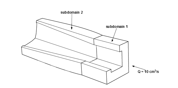
The incompressibility and momentum equations are solved over the computational domain. The domain for the problem is divided into two subdomains (as shown in Figure 5.1: Problem Description) so that the remeshing algorithm can be applied only to the portion of the mesh that is deformed. Subdomain 1 represents the fluid as it enters and is confined by the die. Subdomain 2 corresponds to the extrudate that is in contact with the air (and can deform freely). The main aim of the calculation is to find the location of the free surface (the skin of the extrudate).

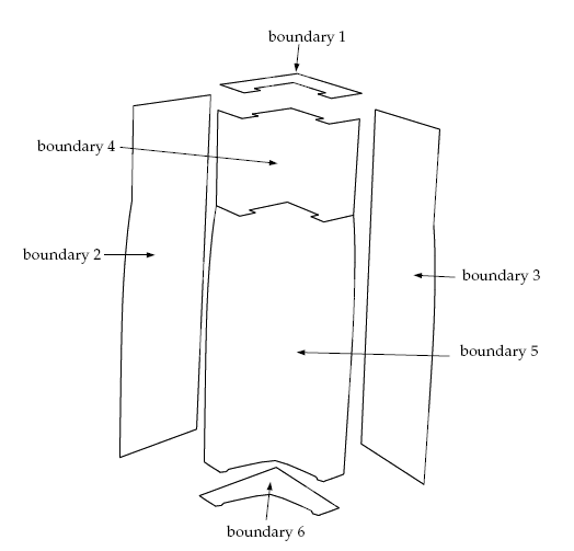
The boundary set for the problem are shown in Figure 5.2: Boundary Set for the Problem, and the conditions at the boundaries of the domains are:

boundary 1: flow inlet, volumetric flow rate = 10 cm³/s
boundary 2: symmetry plane
boundary 3: symmetry plane
boundary 4: zero velocity
boundary 5: free surface
boundary 6: flow exit

Figure 5.2: Boundary Set for the Problem

5.4. Setup and Solution

The following sections describe the setup and solution steps for this tutorial:

5.4.1. Preparation

To prepare for running this tutorial:

Prepare a working folder for your simulation.
Download the direct_extrusion.zip file here .
Unzip the direct_extrusion.zip file you have downloaded to your working folder.
The mesh file dirext.msh can be found in the unzipped folder.
Start Workbench from Start > Ansys 2025 R1 > Workbench 2025 R1.

5.4.2. Project and Mesh

Create a Fluid Flow (Polyflow Classic) analysis system by drag and drop in Workbench.
Save the Ansys Workbench project using File → Save, entering direct-extrusion as the name of the project.
Import the mesh file (dirext.msh).
Double-click the Setup cell to start Polydata.
When Polydata starts, the Create a new task menu item is highlighted, and the geometry for the problem is displayed in the Graphics Display window.

5.4.3. Create a Task for the Model

In the following steps you will define a new task representing the evolution model. Then, you will define a sub-task for the isothermal flow calculation.

Create a task for the model.
Create a new task
1. Select the following options:
  - F.E.M. task
  - Evolution problem(s)
  The complex geometry associated with the free surface of the extrudate introduces nonlinear terms into the kinematic condition equation used to find its location. An evolution scheme is used to handle the nonlinear problem.
2. Click Accept the current setup.
  The Create a sub-task menu item is highlighted.
Create a sub-task for the isothermal flow.
Create a sub-task
1. Select Generalized Newtonian isothermal flow problem.
  A dialog box appears asking for the title of the problem.
2. Enter Direct extrusion as the New value and click OK.
  The Domain of the sub-task menu item is highlighted.
Define the domain where the sub-task applies.
Since this problem involves a free surface, the domain is divided into two subdomains; one for the region near the free surface (SUBDOMAIN_2) and the other for the rest of the domain (SUBDOMAIN_1). In this problem, the sub-task applies to both subdomains, which is the default condition.
Domain of the sub-task
Accept the default selection of both subdomains by clicking Upper level menu.
The Material data menu item is highlighted.

5.4.4. Material Data

Polydata indicates the material properties that are relevant for your sub-task by graying out the irrelevant properties. In this case, viscosity, density, inertia terms, and gravity are available for specification. For this model, define only the viscosity of the material.

Material Data

Click Shear-rate dependence of viscosity.
Click Power law.
The viscosity in this tutorial is given by the power law. For information on power law, see Appendix .
Specify the value for , referred to as “fac” in the graphical user interface (compare the equation at the top of the Power law menu to the equation shown in the Appendix).
Modify fac
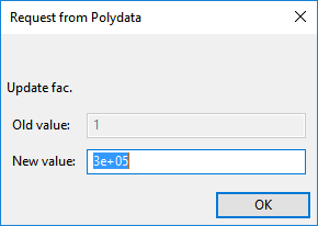
Enter 3e+05 [units: poise] as the New value and click OK.
Retain the default value for , referred to as “tnat” in the graphical user interface.
Modify tnat
Click OK to retain the default value of 1 [units: s].
Specify the value for , referred to as “expo” in the graphical user interface.
Modify expo
Enter 0.75 as the New value and click OK.
Click Upper level menu three times to return to the Direct extrusion menu.
The Flow boundary conditions menu item is highlighted.

5.4.5. Boundary Conditions

In the following steps you will set the conditions at each of the boundaries of the domain. When a boundary set is selected, its location is highlighted in red in the graphics window.

Flow boundary conditions

Set the conditions at the flow inlet (BOUNDARY_1).
1. Select Zero wall velocity (vn=vs=0) along BOUNDARY_1 and click Modify.
2. Click Inflow.
3. Ensure Volumetric flow rate is selected and click Modify volumetric flow rate.
  Polydata prompts you for the volumetric flow rate.
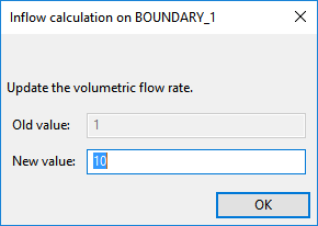
4. Enter 10 [units: cm³/s] as the New value and click OK.
5. Ensure Automatic is selected and click Upper level menu.
  When the Automatic option is selected, Polydata chooses the most appropriate method to compute the inflow condition.
Set the conditions at the first symmetry plane (BOUNDARY_2).
In 2D axisymmetric problems, the axis of symmetry is automatically identified by Polydata, but for 3D flows, you must manually identify a plane of symmetry. The normal velocity () and the tangential force () are set to zero on a symmetry plane. A particle cannot cross the plane ( = 0) due to the symmetry, so the particles flow at the same velocity on both sides of the symmetry plane, leading to a zero tangential force.
1. Select Zero wall velocity (vn=vs=0) along BOUNDARY_2 and click Modify.
2. Click Plane of symmetry (fs=0, vn=0).
Set the conditions at the second symmetry plane (BOUNDARY_3).
1. Select Zero wall velocity (vn=vs=0) along BOUNDARY_3 and click Modify.
2. Click Plane of symmetry (fs=0, vn=0).
Retain the default condition Zero wall velocity (vn=vs=0) along BOUNDARY_4 at the wall of SUBDOMAIN_1 (BOUNDARY_4).
At a solid-liquid interface, the velocity of the liquid is that of the solid surface. Hence the velocity the fluid is assumed to stick to the wall. This is known as the no-slip assumption because the liquid is assumed to adhere to the wall, and hence, has no velocity relative to the wall.
By default, Polydata imposes = = 0 along all boundaries. No action is required to accept the default condition.
Set the conditions at the free surface (BOUNDARY_5).
In a steady-state problem, the velocity field must be tangential to a free surface, since no fluid particles go out of the domain through the free surface. This constraint is called the kinematic condition, = 0. This equation requires an initial condition, that is, the starting line of the free surface. In this problem, the starting line of the free surface is the intersection of boundary 4 and boundary 5 (see Figure 5.2: Boundary Set for the Problem).
1. Select Zero wall velocity (vn=vs=0) along BOUNDARY_5 and click Modify.
2. Click Free surface.
3. Click Boundary conditions on the moving surface.
4. Select No condition along BOUNDARY_4 (the boundary where the free surface starts) and click Modify.
5. Select Position imposed.
6. Click Upper level menu to return to the Boundary conditions on the moving surface menu.
7. Click Upper level menu two times to return to the Flow boundary conditions menu.
Set the conditions at the flow exit (BOUNDARY_6).
It is assumed that a uniform velocity profile is reached at the exit. The melt is not subjected to any externally applied stress at the exit, so the condition of zero normal and tangential forces is selected.
1. Select Zero wall velocity (vn=vs=0) along BOUNDARY_6 and click Modify.
2. Click Normal and tangential forces imposed (fn, fs).
3. Accept the default value of 0 for the normal force, , by clicking Upper level menu.
4. Accept the default value of 0 for the tangential force, , by clicking Upper level menu.
5. Click Upper level menu to return to the Direct extrusion menu.
  The Global remeshing menu item is highlighted.

5.4.6. Remeshing

This model involves a free surface, whose shape is unknown a priori, which will be calculated together with the flow equations. A portion of the mesh is affected by the relocation of this boundary, so a remeshing technique is applied on this part of the mesh. The free surface is entirely contained within subdomain 2, therefore only subdomain 2 is affected by the relocation of the free surface.

Global remeshing

Specify the region where the remeshing is to be performed (SUBDOMAIN_2).
In general, only one local remeshing is required for direct extrusion simulations. It becomes necessary to define multiple local remeshings for inverse extrusion simulations. A single local remeshing is sufficient for this case.
1–st local remeshing
1. Select SUBDOMAIN_1 and click Remove.
  SUBDOMAIN_1 is moved from the top list to the bottom list, indicating that only SUBDOMAIN_2 will be remeshed.
2. Click Upper level menu.
Define the parameters for the remeshing method.
The purpose of the remeshing technique is to relocate internal nodes according to the displacement of boundary nodes due to the motion of the free surface, since a part of the mesh is deformed. For 3D extrusion problems where large deformations of the extrudate are expected, the optimesh remeshing technique is recommended. For information on optimesh remeshing technique, refer to the Appendix.
Optimesh-3D (extrusion only)
1. Specify the initial plane for the optimesh remeshing technique, by selecting SUBDOMAIN_1 and clicking Modify.
  1. Select Part of inlet section.
  2. Select Upper level menu.
2. Specify the final plane for remeshing technique, by selecting BOUNDARY_6 and clicking Modify.
  1. Select Part of outlet section.
  2. Select Upper level menu twice.
  Polydata asks if you want to change from the surface kinematic condition to the line kinematic condition.
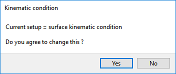
3. Click Yes to use the line kinematic condition.
  The line kinematic condition is recommended for extrusion problems, and must be used in combination with the optimesh remeshing technique.
4. Click Accept the current setup in the Element distortion check menu.
  In complex extrusion simulations, the finite element mesh can undergo great deformations. The Element distortion check menu deals with the detection of all possible distortions of the elements.
5. Click Upper level menu two times.
  F.E.M. Task 1 menu is displayed.

5.4.7. Numerical Parameters

All information relevant to iterative schemes (for the F.E.M. task calculations) can be modified in the Numerical parameters menu.

Numerical parameters

Click Enable evolution on moving boundaries to enable the evolution scheme.
For information on the evolution scheme, see Appendix.
Specify the evolution parameters.
Modify the evolution parameters
1. Define the starting solution for the iterative scheme in the calculation of the free surface location.
  The first calculation is performed at . Increase the value of the initial increment of () to reduce the number of evolution steps and to speed up the calculation.
  Modify the initial value of delta-S
  Polydata prompts you for the initial value of .
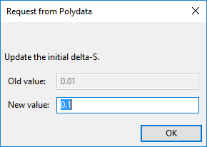
2. Enter 0.1 for the New value and click OK.
3. Click Upper level menu to return to the Numerical parameters menu.
Click Upper level menu two times to return to the top-level Polydata menu.

5.4.8. Outputs

After Polyflow Classic calculates a solution, it can save the results in several different formats. Choose the one that is appropriate for your postprocessor. In this case, save the outputs in IGES format, as well as the default format for CFD-Post.

Outputs

Retain the default output (CFD-Post) and click Enable Iges file output.
The default CFD-Post output is used for postprocessing with CFD-Post. The IGES output contains the modified geometry of the extrudate (after remeshing) calculated at every step of the evolution procedure. For information on IGES output, see Appendix.
Polydata asks you to confirm the current system units and fields that are to be saved to the results file for postprocessing.
Specify the system of units for the simulation.
1. Click Modify system of units.
2. Select Set to metric_cm/g/s/A+Celsius.
3. Click Upper level menu three times.
  The top-level Polydata menu is displayed.

5.4.9. Save and Exit Polydata

Save and exit

Polydata asks you to confirm fields that are to be saved to the results file for postprocessing.

Click Accept current setup in the Convergence strategies menu.
Click Accept in the Field Management menu.
This confirms that the default Current field(s) are correct.
Click Continue.
This accepts the default names for graphical output files (cfx.res) that are to be saved for postprocessing, and for the Polyflow Classic format results file (res).

5.4.10. Solution

Run Polyflow Classic to calculate a solution for the model you just defined using Polydata.

Run Polyflow Classic by right-clicking the Solution cell of the simulation and selecting Update.
This executes Polyflow Classic using the data file as standard input, and writes information about the problem description, calculations, and convergence to a listing file (polyflow.lst).
Check for convergence in the listing file.
1. Right-click the Solution cell and select Listing Viewer....
  Workbench opens the View listing file dialog box, which displays the listing file.
2. It is a common practice to confirm that the solution proceeded as expected by looking for the following printed at the bottom of the listing file:
```
The computation succeeded.
```

5.4.11. Postprocessing

Use CFD-Post to view the results of the Polyflow Classic simulation.

Double-click the Results tab in the Polyflow Classic analysis system. This will start CFD-Post and read the results files saved by Polyflow Classic. CFD-Post reads the mesh information and the solution fields that were saved to the results file.
Display the velocity distribution on the boundaries.
Deselect Wireframe in the Outline tree tab, under User Locations and Plots.
1. Click the Insert menu and select Contour or click the button.
2. Click OK to accept the default name (Contour 1) and display the details view below the Outline tab.
3. Perform the following steps in the Geometry tab of the details view of Contour 1:
  1. Click the button next to Locations.
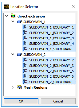
  2. Select all topological entities under SUBDOMAIN_1 and SUBDOMAIN_2 in the Location Selector dialog box (use Shift for multiple selection) and click OK.
  3. Select VELOCITIES from the Variable drop-down list (or by clicking ).
  4. Click Apply.
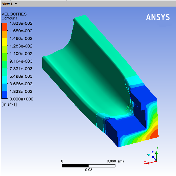
4. Rotate the image so that you can see the fluid at the inlet of the die, as shown in Figure 5.3: Contours of Velocity Magnitude.
Figure 5.3: Contours of Velocity Magnitude

Observe that the velocity is zero along the die wall, as expected, and there is a fully developed profile at the inlet of the die. At the die outlet, the velocity profile changes to become constant throughout the extrudate cross-section. The transition between these two states can be seen in the first third of the extrudate.
Display contours of velocity in cross-sections.
1. Deselect the contours previously defined.
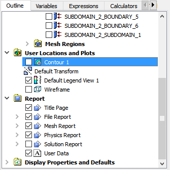
  In the Outline tree tab, under User Locations and Plots, deselect Contour 1.
2. Create the cross-sectional planes, at Z = 0, 3, 7, and 20 cm.
  1. Select Plane from the Location drop-down menu ( ).
  2. Click OK to accept the default name (Plane 1) and display the details view below the Outline tab.
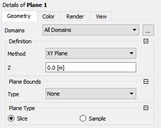
  3. In the Geometry tab of the details view, ensure XY Plane is selected from the Method drop-down list.
  4. Enter 0 for Z.
  5. Click Apply.
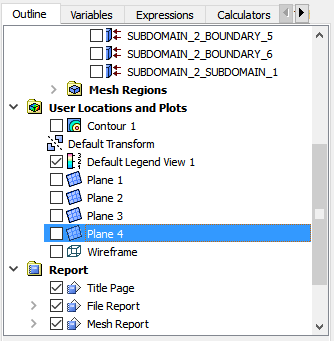
  6. Repeat steps 3.b.i.–v. for the other planes, at Z = 0.03, 0.07, and 0.1999 m.
  7. In the Outline tree tab, under User Locations and Plots, deselect Plane 1, Plane 2, Plane 3, and Plane 4.
3. Display the contours.
  1. Click the Insert menu and select Contour or click the button.
  2. Click OK to accept the default name (Contour 2) and display the details view below the Outline tab.
  3. In the Outline tree tab under User Locations and Plots, select Wireframe.
  4. In the Geometry tab of the details view of Contour 2, click the button next to Locations.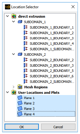
  5. Select all planes under User Locations and Plots (use Shift for multiple selection).
  6. Click OK.
  7. Select VELOCITIES from the Variable drop-down list (or click ).
  8. In the Render tab, disable Lighting.
  9. Click Apply.
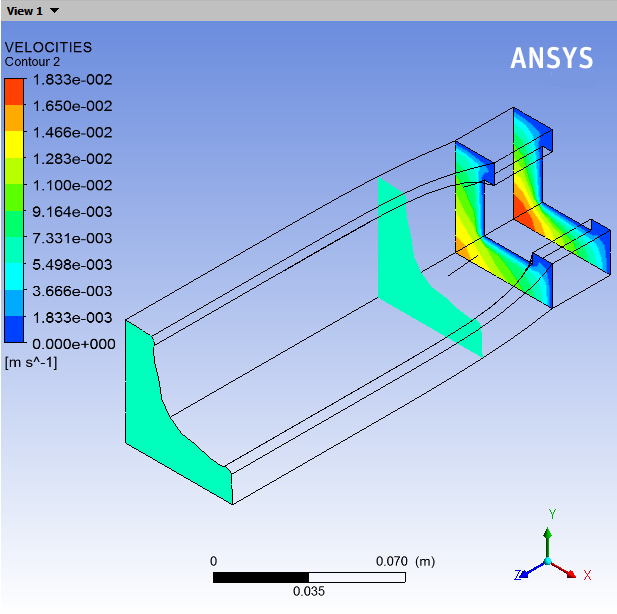
Figure 5.4: Velocity Profiles at Cross-Sections shows the velocity profiles at the flow inlet, the flow outlet, and at the planes just before and just after the die exit.
Figure 5.4: Velocity Profiles at Cross-Sections

Compare the velocity profile within the die to the velocity profile just after the die exit at the end of the computational domain. In the die the flow is fully developed. In the extrudate, far away from the die exit, the velocity profile is flat. That is, all the particles in a cross-sectional plane are at the same speed. Just after the die exit, there is a transitional zone where the velocity profile is reorganized. The velocity profile on the plane Z = 7 cm is no longer fully developed, but it is not yet flat either. The velocity rearrangement is the source of the deformation of the extrudate.
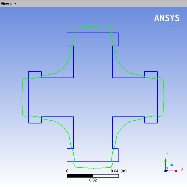
Compare the cross-sectional shape of the extrudate with the die.
1. Simplify the display.
  In the Outline tree tab, under User Locations and Plots, deselect Contour 2 and Wireframe.
2. Display the die shape using a polyline.
  1. Select Polyline from the Location drop-down menu ( ).
  2. Click OK to accept the default name (Polyline 1) and display the details view below the Outline tab.
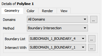
  3. In Geometry tab of the details view, select Boundary Intersection from the Method drop-down list.
  4. Click next to Boundary List and select SUBDOMAIN_1_BOUNDARY_4. Click OK to close the Location Selector dialog box.
  5. Select SUBDOMAIN_1_BOUNDARY_1 from the Intersect With drop-down list.
  6. In the Color tab, click next to Color and select dark blue.
  7. Click Apply.
3. Display the extrudate shape using a polyline.
  1. Select Polyline from the Location drop-down menu ( ).
  2. Click OK to accept the default name (Polyline 2) and display the details view below the Outline tab.
  3. In Geometry tab of the details view, select Boundary Intersection from the Method drop-down list.
  4. Select SUBDOMAIN_2_BOUNDARY_5 from the Boundary List drop-down list.
  5. Select SUBDOMAIN_2_BOUNDARY_6 from the Intersect With drop-down list.
  6. Click Apply.
4. Right-click in the graphic window and select View From +Z under Predefined Camera.
  This allows you to compare the size and shape of the flow inlet with that of the flow outlet without distortion due to perspective.
Restore the symmetry.
1. Click the Insert menu and select Instance Transform, or click the button.
2. Click OK to accept the default name (Instance Transform 1) and display the details view below the Outline tab.
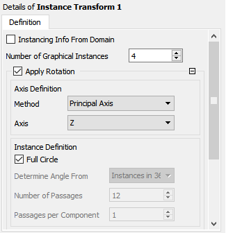
3. Perform the following steps in the details view of Instance Transform 1:
  1. Disable Instancing Info From Domain.
  2. Set Number of Graphical Instances to 4.
  3. Ensure Apply Rotation is selected.
  4. Ensure Method is set to Principal Axis and Z is selected from the Axis drop-down list.
  5. Enable Full Circle under Instance Definition.
  6. Click Apply.
4. In the Outline tree tab, under User Locations and Plots, right-click Polyline 1 and click Edit (or double-click Polyline 1).
5. In the View tab, scroll down and enable Apply Instancing Transform.
6. Select Instance Transform 1 from the Transform drop-down list.
7. Click Apply.
8. In the Outline tree tab, under User Locations and Plots, right-click Polyline 2 and click Edit (or double-click Polyline 2).
9. Repeat steps 5.e.–g.
You can use the central-mouse button to zoom in and out. This allows you to compare the size and shape of the flow inlet with that of the flow outlet without distortion due to perspective.
You can also click the fit view button ( ) to properly center the image.
Figure 5.5: Swelling of the Extrudate

The deformations come from the rearrangement of the velocity profile. Particles coming from high-speed regions in the die must slow down, while particles coming from low-speed regions must accelerate. Observe that the central part of the cross, where the fluid easily flows in the die, is enlarged in the extrudate, while the extremities of the branches are smaller in the extrudate. Since the combined effect of cross-sectional expansions and reductions is very difficult to guess, a numerical simulation is necessary for a moderate to high complexity die.

5.5. Summary

This tutorial introduced the concept of a direct extrusion problem. You solved the problem using a specific 3D geometry for the die, made suitable assumptions about the physics of the problem, and analyzed the factors affecting the extrudate shape. The nonlinear problem was solved using an evolution technique to reach the convergence.

5.6. Appendix

The appendix contains the following sections:

5.6.1. Power Law

The power law exhibits shear thinning (reduction in the viscosity with an increase in shear rate) that is a characteristic of many polymers. The viscosity in this tutorial is given by the power law:

(5–1)

where:

= consistency factor

= power-law index

= natural time

is included in the equation to make the units consistent.

5.6.2. Optimesh Remeshing Technique

The optimesh remeshing technique requires the direction of extrusion to be parallel to the , , or axis, and all slices into which the remeshing domain is cut must be perpendicular to the extrusion axis.

The domain to be remeshed is cut into a series of 2D slices (planes) in a direction perpendicular to the direction of extrusion, and each plane will be remeshed independently. For this process, Polyflow Classic requires the selection of the initial plane and the final plane. In this problem, the initial plane is the intersection of SUBDOMAIN_2 with SUBDOMAIN_1, and the final plane is the intersection of SUBDOMAIN_2 with the flow exit (boundary 6).

5.6.3. Evolution Scheme

The kinematic equation introduces nonlinear terms in the problem that might lead to convergence difficulties. An evolution scheme is available in Polyflow Classic to solve such highly nonlinear problems. Start the calculation with a reduced value of the parameter(s) causing the nonlinearity. Beginning with the first solution, Polyflow Classic increments the parameter(s) causing the nonlinearity and computes a second solution. Starting from this new solution, Polyflow Classic increments the parameter(s) again and computes a third solution. Following this procedure, Polyflow Classic increases the value of each parameter up to its nominal value. In Polyflow Classic, this procedure is fully automated; the increments are automatically adapted according to the results of previous calculations. Polyflow Classic uses an evolution variable that is incremented during the evolution scheme. S starts at an initial value of and is increased to a final value of . Each parameter that you want to evolve is defined as .

5.6.4. IGES Output

An IGES output allows you to import the final geometry into a CAD program. This is useful when you are designing a die because you want to be able to manufacture the die predicted by the calculation. In the present case, you can compare the final shape of the predicted extrudate in an IGES format with the desired shape.