


This tutorial is divided into the following sections:
This tutorial illustrates the simulation of a 3D extrusion process. Due to the velocity rearrangement that occurs at the die exit, the shape of the extrudate is usually different from the die lip cross-section. Polyflow Classic is capable of handling 3D free surfaces, so it can predict the extrudate shape that corresponds to a given die geometry under prescribed operating conditions.
In this tutorial you will learn how to:
Create a sub-task to define a 3D extrusion problem.
Set material properties and boundary conditions for a 3D extrusion problem.
Select a remeshing method.
This tutorial assumes that you are familiar with the menu structure in Polydata and Workbench and that you have solved or read 2.5D Axisymmetric Extrusion. Some steps in the setup procedure will not be shown explicitly.
This problem deals with the flow of a Newtonian fluid through a three-dimensional die. Due to the symmetry of the problem (the cross-section of the die is a square), the computational domain is defined for a quarter of the geometry and two planes of symmetry are defined.
The melt enters the die as shown in Figure 4.1: Problem Description at a flow rate of  = 10 cm3/s (a quarter of the actual flow rate) and the extrudate is obtained
at the exit. At the end of the computational domain, it is assumed
that the extrudate is fully deformed and that it will not deform any
further. It is assumed that subdomain 2 is long enough to account
for all the deformation of the extrudate.
= 10 cm3/s (a quarter of the actual flow rate) and the extrudate is obtained
at the exit. At the end of the computational domain, it is assumed
that the extrudate is fully deformed and that it will not deform any
further. It is assumed that subdomain 2 is long enough to account
for all the deformation of the extrudate.
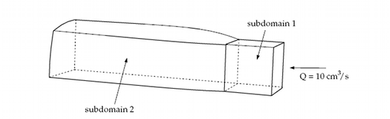
The incompressibility and momentum equations are solved over the computational domain. The domain for the problem is divided into two subdomains (as shown in Figure 4.1: Problem Description) so that the remeshing algorithm can be applied only to the portion of the mesh that will be deformed. The subdomain 1 represents the die where the fluid is confined. The subdomain 2 corresponds to the extrudate that is in contact with the air and can deform freely. The main aim of the calculation is to find the location of the free surface (the skin of the extrudate).
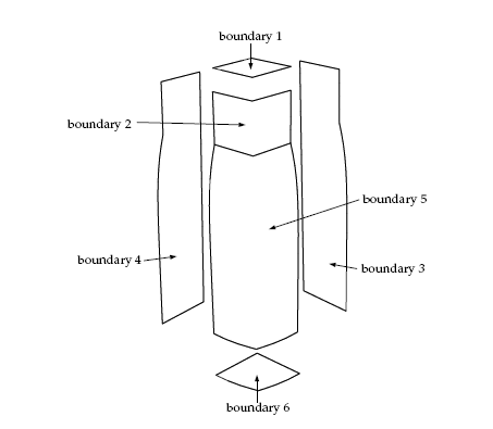
The boundary sets for the problem are shown in Figure 4.2: Boundary Sets for the Problem, and the conditions at the boundaries of the domains are as follows.
boundary 1: flow inlet, volumetric flow rate
 = 10 cm3/s
boundary 2: zero velocity
boundary 3: symmetry plane
boundary 4: symmetry plane
boundary 5: free surface
boundary 6: flow exit
To prepare for running this tutorial:
Prepare a working folder for your simulation.
Download the
3d_extrusion.zipfile here .Unzip the
3d_extrusion.zipfile you have downloaded to your working folder.The mesh file
ext3d.mshcan be found in the unzipped folder.Start Workbench from .
The following sections describe the setup and solution steps for this tutorial:
Create a Fluid Flow (Polyflow Classic) analysis system by drag and drop in Workbench.
Save the Ansys Workbench project using File → , entering
3D-extrusionas the name of the project.Import the mesh file (
ext3d.msh).Double-click the Setup cell to start Polydata.
When Polydata starts, the Create a new task menu item is highlighted, and the geometry for the problem is displayed in the Graphics Display window.
Define a new task representing the 3D steady-state model, then define a sub-task for the isothermal flow calculation.
Create a task for the model.
 Create a new task
Retain the following (default) options:
F.E.M. task
Steady-state problem(s)
This problem is a 3D simulation of the extrusion process, that is, a three-dimensional geometry is assumed for the die. A Cartesian (x,y,z) reference frame is used for the 3D calculations. A steady-state condition is assumed for the problem.
Click Accept the current setup.
The Create a sub-task menu item is highlighted.
Create a sub-task for the isothermal flow.
Create a sub-task
Select Generalized Newtonian isothermal flow problem.
A dialog box appears asking for the title of the problem.
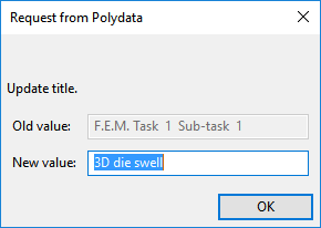
Enter
3D die swellas the New value and click .The Domain of the sub-task menu item is highlighted.
Define the domain where the sub-task applies.
Since this problem involves a free surface, the domain is divided into two subdomains; one for the region near the free surface (subdomain 2) and the other for the rest of the domain (subdomain 1). In this problem, the sub-task applies to both subdomains, which is the default condition.
Domain of the sub-task
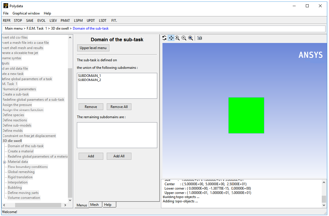
Accept the default selection of both subdomains (SUBDOMAIN_1 and SUBDOMAIN_2) by clicking Upper level menu.
The Material data menu item is highlighted.
Polydata indicates which material properties are relevant for the sub-task by graying out the irrelevant properties. In this case, viscosity, density, inertia terms, and gravity are available for specification. For this model you will only define the viscosity of the material.
![]() Material Data
Material Data
Click Shear-rate dependence of viscosity.
Click Cross law.
The Cross law exhibits shear-thinning (the decrease in viscosity as the shear rate increases) that is a characteristic of many polymers. The viscosity in this tutorial is given by the Cross law:

(4–1)
where:
 = zero shear-rate viscosity = 85000 poise
  = natural time = 0.2 s
 = Cross law index = 0.3
 = shear rate
Specify the value
 , referred to as “fac” in the graphical
user interface (compare the equation at the top of the Cross
law menu to Equation 4–1).
Modify fac
, referred to as “fac” in the graphical
user interface (compare the equation at the top of the Cross
law menu to Equation 4–1).
Modify fac

Enter
85000[units: poise] as the New value and click .Specify the value for
 , referred to as “tnat”
in the graphical user interface.
Modify tnat
, referred to as “tnat”
in the graphical user interface.
Modify tnat
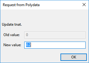
Enter
0.2[units: s] as the New value and click .Specify the value for
 , referred to as “expom”
in the graphical user interface.
Modify expom
, referred to as “expom”
in the graphical user interface.
Modify expom
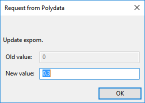
Enter
0.3as the New value and click .Select Upper level menu three times to return to the 3D die swell menu.
The Flow boundary conditions menu item is highlighted.
In the following steps you will set the conditions at each of the boundaries of the domain. When a boundary set is selected, its location is highlighted in red in the graphics window.
![]() Flow boundary conditions
Flow boundary conditions
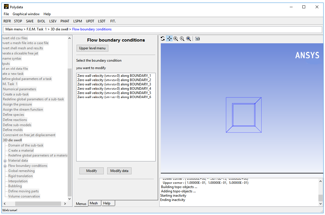
Set the conditions at the flow inlet (BOUNDARY_1).
Select Zero wall velocity (vn=vs=0) along BOUNDARY_1 and click .
Click Inflow.
Retain the default settings, Automatic and Volumetric flow rate.
Click Modify volumetric flow rate.
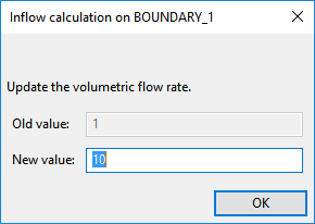
Enter
10[units: cm3/s] as the New Value and click .When the Automatic option is selected, Polydata automatically chooses the most appropriate method to compute the inflow condition.
Click Upper level menu.
Retain the default condition Zero wall velocity (vn=vs=0) along BOUNDARY_2 at the wall of SUBDOMAIN_1 (BOUNDARY_2).
At a solid-liquid interface, the velocity of the liquid is that of the solid surface. Hence the fluid is assumed to stick to the wall. This is known as the no-slip condition because the liquid is assumed to adhere to the wall, and hence, has no velocity relative to the wall.
By default, Polydata imposes
 =
=  = 0 along all boundaries. No action
is required to accept the default condition.
= 0 along all boundaries. No action
is required to accept the default condition.
Set the conditions at the first symmetry plane (BOUNDARY_3).
In 2D axisymmetric problems, Polydata automatically identifies the axis of symmetry, but for 3D flows, you must manually identify a plane of symmetry.
The normal velocity (
 ) and the tangential force (
 ) are set to zero on a symmetry plane. A
particle cannot cross the plane (
) are set to zero on a symmetry plane. A
particle cannot cross the plane ( = 0) due to the symmetry, so the
particles flow at the same velocity on both sides of the symmetry
plane, leading to a zero tangential force.
= 0) due to the symmetry, so the
particles flow at the same velocity on both sides of the symmetry
plane, leading to a zero tangential force.
Select Zero wall velocity (vn=vs=0) along BOUNDARY_3 and click .
Click Plane of symmetry (fs=0, vn=0).
Set the conditions at the second symmetry plane (BOUNDARY_4).
Select Zero wall velocity (vn=vs=0) along BOUNDARY_4 and click .
Click Plane of symmetry (fs=0, vn=0).
Set the conditions at the free surface (BOUNDARY_5).
In a steady-state problem, the velocity field must be tangential to a free surface, since no fluid particles go out of the domain through the free surface. This constraint is called the kinematic condition,
 . This equation requires an initial condition, that
is, the starting line of the free surface. In the current problem,
the starting line of the free surface is the intersection of boundary
2 and boundary 5 (see Figure 4.2: Boundary Sets for the Problem).
. This equation requires an initial condition, that
is, the starting line of the free surface. In the current problem,
the starting line of the free surface is the intersection of boundary
2 and boundary 5 (see Figure 4.2: Boundary Sets for the Problem).
Select Zero wall velocity (vn=vs=0) along BOUNDARY_5 and click .
Click Free surface.
Click Boundary conditions on the moving surface.
Select No condition along BOUNDARY_2 and click .
Select Position imposed.
Click Upper level menu.
Click Upper level menu to return to the Kinematic condition menu.
Click Upper level menu to return to the Flow boundary conditions panel.
Set the conditions at the flow outlet (BOUNDARY_6).
It is assumed that a uniform velocity profile is reached at the exit. The melt is not subjected to any externally applied stress at the exit, so the condition of zero normal and tangential forces is selected.
Select Zero wall velocity (vn=vs=0) along BOUNDARY_6 and click .
Click Normal and tangential forces imposed (fn, fs).
Accept the default value of 0 for the normal force,
 , by clicking Upper level menu.
Accept the default value of 0 for the tangential force,
 , by clicking Upper level menu.
Click Upper level menu at the top of the Flow boundary conditions panel.
This model involves a free surface, whose shape is unknown a priori, which will be calculated together with the flow equations. A portion of the mesh is affected by the relocation of this boundary, so a remeshing technique is applied on this part of the mesh. The free surface is entirely contained within subdomain 2, therefore only subdomain 2 is affected by the relocation of the free surface.
![]() Global remeshing
Global remeshing
Specify the region where the remeshing is to be performed (SUBDOMAIN_2).
In general, only one local remeshing is required for direct extrusion simulations. It becomes necessary to define multiple local remeshings for inverse extrusion simulations. A single local remeshing is sufficient for this case.
1–st local remeshing
Select SUBDOMAIN_1 and click .
SUBDOMAIN_1 is moved from the top list to the bottom list, indicating that only SUBDOMAIN_2 will be remeshed.
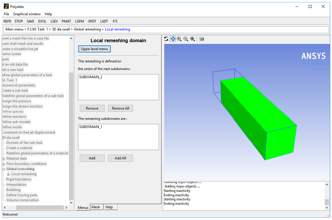
Click Upper level menu.
Define the parameters for the remeshing method.
The purpose of the remeshing technique is to relocate internal nodes according to the displacement of boundary nodes due to the motion of the free surface, since a part of the mesh is deformed. For 3D extrusion problems where large deformations of the extrudate are expected, the optimesh remeshing technique is recommended
The optimesh remeshing technique requires the direction of extrusion to be parallel to the
 ,
,  , or
, or  axis, and all slices into which
the remeshing domain is cut must be perpendicular to the extrusion
axis.
axis, and all slices into which
the remeshing domain is cut must be perpendicular to the extrusion
axis.
The domain to be remeshed is cut into a series of 2D slices (planes) in a direction perpendicular to the direction of extrusion, and each plane is remeshed independently. For this process, Polyflow Classic requires the selection of the initial plane and the final plane. In this problem, the initial plane is the intersection of subdomain 2 with subdomain 1, and the final plane is the intersection of subdomain 2 with the flow exit (boundary 6).
Optimesh-3D (extrusion only)
Specify the initial plane for the optimesh remeshing technique, by selecting SUBDOMAIN_1 and clicking .
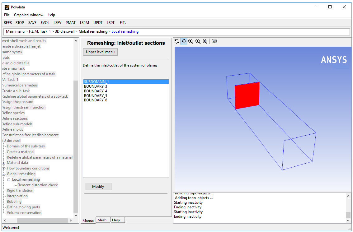
Select Part of inlet section.
Select Upper level menu.
Specify the final plane for the optimesh remeshing technique, by selecting BOUNDARY_6 and clicking .
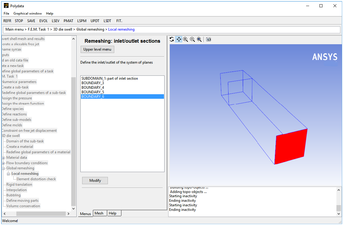
Select Part of outlet section.
Select Upper level menu.
Click Upper level menu.
Polydata asks if you want to change from the surface kinematic condition to the line kinematic condition.
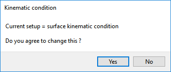
Click to use the line kinematic condition.
The line kinematic condition is recommended for extrusion problems, and should be used in combination with the optimesh remeshing technique.
Click Upper level menu three times.
The top-level Polydata menu is displayed.
![]() Save and exit
Save and exit
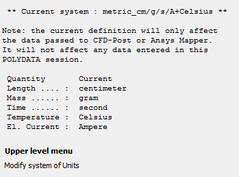
Polydata asks you to confirm the current system units and fields that are to be saved to the results file for postprocessing.
Specify the system of units for the simulation.
Click Modify system of units.
Select Set to metric_cm/g/s/A+Celsius
Click Upper level menu twice.
Click Accept current setup in the Convergence strategies menu.
Click in the Field Management menu.
This confirms that the default Current field(s) are correct.
Click Continue.
This accepts the default names for graphical output files (
cfx.res) that are to be saved for postprocessing, and for the Polyflow Classic format results file (res).
Run Polyflow Classic to calculate a solution for the model you just defined using Polydata.
Run Polyflow Classic by right-clicking the Solution cell of the simulation and selecting Update.
This executes Polyflow Classic using the data file as standard input, and writes information about the problem description, calculations, and convergence to a listing file (
polyflow.lst).Check for convergence in the listing file.
Right-click the Solution cell and select Listing Viewer....
Workbench opens the View listing file dialog box, which displays the listing file.
It is a common practice to confirm that the solution proceeded as expected by looking for the following printed at the bottom of the listing file:
The computation succeeded.
Use CFD-Post to view the results of the Polyflow Classic simulation.
Double-click the Results cell in the Workbench analysis and read the results files saved by Polyflow Classic.
CFD-Post reads the solution fields that were saved to the results file.
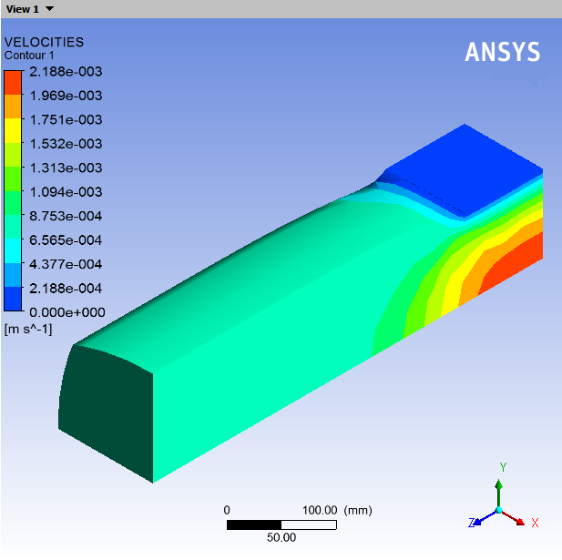
Display the velocity distribution on the boundaries.
Click the Insert menu and select Contour or click the
 button.
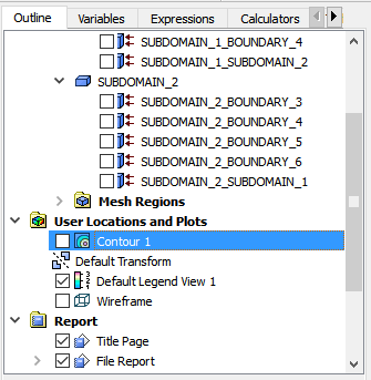
 Click to accept the default name (Contour 1) and display the details view below the Outline tab.
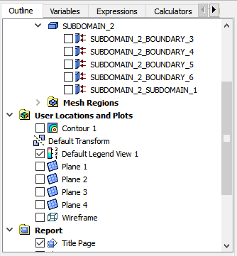
In the Outline tree tab, under User Locations and Plots, deselect Wireframe.
Perform the following steps in the details view of Contour 1:
In the Geometry tab, click the
 button next to Locations.
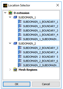
Select all topological entities under SUBDOMAIN_1 and SUBDOMAIN_2 in the Location Selector dialog box (use Shift) and click .
Select VELOCITIES from the Variable drop-down list (or by clicking
).In the Render tab, deselect Show Contour Lines.
Click Apply.
In Figure 4.3: Contours of Velocity Magnitude, the velocity is zero along the die wall (as expected) and there is a fully developed profile at the inlet of the die. At the die outlet, the velocity profile changes to become constant throughout the extrudate cross-section. The transition between these two states can be seen in the beginning section of the extrudate.
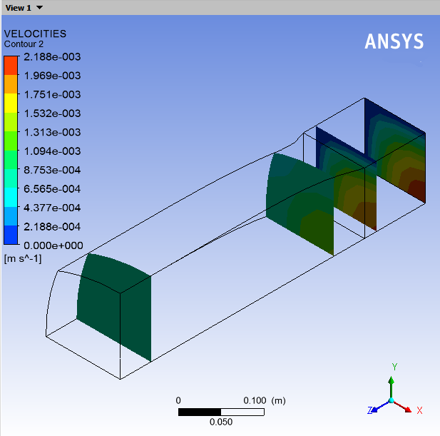
Display contours of velocity in cross-sections.
Deselect Contour 1 in the Outline tree tab under User Locations and Plots.
Create the cross-section planes, at Z = 0, 0.08, 0.15, 0.45 m.
Select Plane from the Location drop-down menu (
 ).
).Click to accept the default name (Plane 1) and display the details view below the Outline tab.
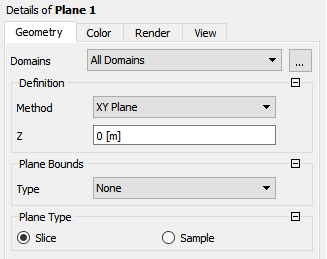
In the Geometry tab of the details view of Plane 1, ensure XY Plane is selected from the Method drop-down list.
Enter
0for Z.Click .
Repeat steps 3.b.i.–v. for the other planes, at Z =
0.08,0.15, and0.45m.In the Outline tree tab, under User Locations and Plots, deselect Plane 1, Plane 2, Plane 3, and Plane 4.
Click the Insert menu and select Contour or click the
button. Click to accept the default name (Contour 2) and display the details view below the Outline tab.
In the Outline tree tab under User Locations and Plots, select Wireframe.
Perform the following steps in the details view of Contour 2:
In the Geometry tab, click the
button next to Locations.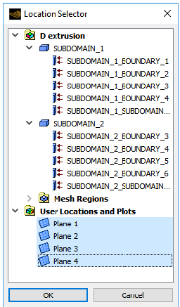
Select all planes under User Locations and Plots (use Shift for multiple selection).
Click .
Select VELOCITIES from the Variable drop-down list (or click
).In the Render tab, deselect Show Contour Lines.
Click Apply.
Velocity profiles at the flow inlet, the flow outlet, and planes just before and just after the die exit are displayed (Figure 4.4: Velocity Profiles at Cross-Sections). Compare the velocity profile within the die to the velocity profile just after the die exit at the end of the computational domain. In the die the flow is fully developed. The velocity profile is flat in the extrudate, far away from the die exit; all the particles in the cross-section plane are at the same velocity. Just beyond the die exit, in the transitional zone, the velocity profile is reorganized. The velocity profile on the plane
 = 15 is no longer fully developed,
but it is not yet flat either. The velocity rearrangement is the source
of the deformation of the extrudate.
= 15 is no longer fully developed,
but it is not yet flat either. The velocity rearrangement is the source
of the deformation of the extrudate.
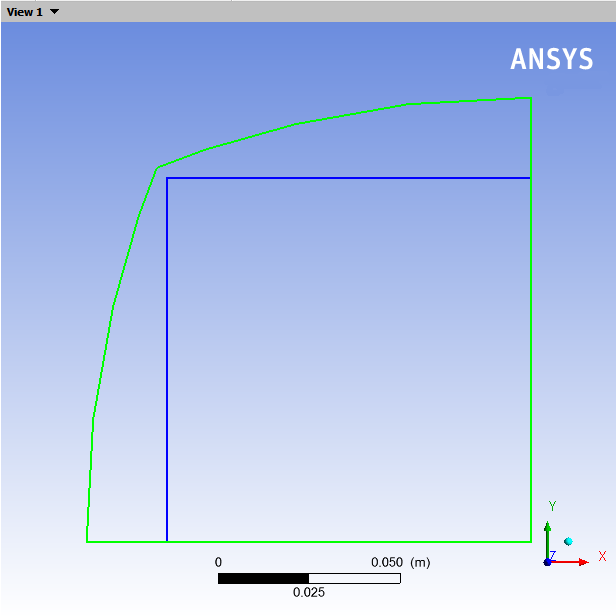
Compare the cross-section shape of the extrudate with die.
Simplify the display.
In the Outline tree tab, under User Locations and Plots, deselect Contour 2 and Wireframe.
Display the die shape using a polyline.
Select Polyline from the Location drop-down menu (
). Click to accept the default name (Polyline 1) and display the details view below the Outline tab.
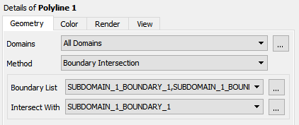
In the Geometry tab of the details view, select Boundary Intersection from the Method drop-down list.
Click
next to Boundary List and
select SUBDOMAIN_1_BOUNDARY_2, SUBDOMAIN_1_BOUNDARY_3, SUBDOMAIN_1_BOUNDARY_4 (use Shift for multiple selection). Click to close
the Location Selector dialog box.Select SUBDOMAIN_1_BOUNDARY_1 from the Intersect With drop-down list.
Under the Color tab, click
next to Color and select dark blue.Click .
Display the extrudate shape using a polyline.
Select Polyline from the Location drop-down menu (
). Click to accept the default name (Polyline 2) and display the details view below the Outline tab.
In the Geometry tab of the details view, select Boundary Intersection from the Method drop-down list.
Click
next to Boundary List and
select SUBDOMAIN_2_BOUNDARY_3, SUBDOMAIN_2_BOUNDARY_4, SUBDOMAIN_2_BOUNDARY_5 (use Shift for multiple selection).Select SUBDOMAIN_2_BOUNDARY_6 from the Intersect With drop-down list.
Click .
On the axis triad in the graphics window click +Z to view from Z-direction.
This allows you to compare the size and shape of the flow inlet with that of the flow outlet without distortion due to perspective.
Since the model involves a generalized Newtonian fluid, there are no viscoelastic effects. The swelling (Figure 4.5: Swelling of the Extrudate) is only due to reorganization of the velocity profile at the die exit. Fluid from the high-speed region moves to the low-speed region and pushes the free surface to the exterior.
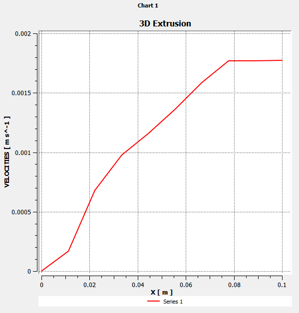
Create a 2D plot on the diagonal of the die.
Define the line of the plot with the points (0.0, 0.1, 0.1) and (0.1, 0.0, 0.1).
These values are in meters.
Select Line from the Location drop-down menu (
). Click to accept the default name (Line 1) and display the details view below the Outline tab.
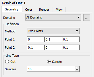
Enter
0,0.1,0.1for Point 1 and0.1,0,0.1for Point 2.Click .
Create a plot.
Click the chart button
 .
. Click to accept the default name (Chart 1) and display the details view below the Outline tab.
In the General tab of the details view, ensure XY - Line is selected for Type, and enter
3D
          Extrusion
for Title.In the Data Series tab, for Series 1, select Line 1 from the Locations drop-down list (or by clicking the
button).In the X Axis tab, select X from the Variable drop-down list.
In the Y Axis tab, select VELOCITIES from the Variable drop-down list.
Click .
The shear-thinning introduced by the Cross law is not clearly visible in Figure 4.6: Velocity Magnitude Along a Diagonal of Die Exit Section due to the large finite elements along the die wall. The mesh should be refined in that zone.
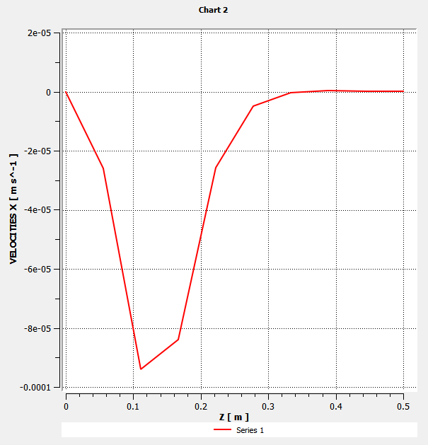
Plot X-velocity close to center of the die.
Define the line of the plot with the points (0.08, 0.02, 0.00) and (0.08, 0.02, 0.50).
Select Line from the Location drop-down menu (
). Click to accept the default name (Line 2) and display the details view below the Outline tab.
Enter
0.08,0.02,0for Point 1 and0.08,0.02,0.5for Point 2.Click .
Create a plot.
Click the chart button
. Click to accept the default name (Chart 2) and display the details view below the Outline tab.
In the General tab of the details view, ensure XY is selected for Type, and disable Display Title.
In the Data Series tab, select Line 2 from the Locations drop-down list for Series 1.
In the X Axis tab, select Z from the Variable drop-down list.
In the Y Axis tab, select VELOCITIES X from the Variable drop-down list.
Click .
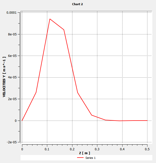
Plot Y-velocity close to the center of the die.
In the Y Axis tab of the details of Chart 2, select VELOCITIES Y from the Variable drop-down list.
Click .
Plot Z-velocity close to the center of the die.
In the Y Axis tab of the details view of Chart 2, select VELOCITIES Z from the Variable drop-down list.
Click .
Figure 4.9: Velocities Along a Line Close to the Center of the Die shows that the flow slows down (
 decreases) after the die exit. Meanwhile,
particles travel from the center of the extrudate toward the edge,
creating the swelling of the extrudate. Figure 4.7: X-Velocities Along a Line Close to the Center of the Die and Figure 4.8: Y-Velocities Along a Line Close to the Center of the Die show that the peak values of
decreases) after the die exit. Meanwhile,
particles travel from the center of the extrudate toward the edge,
creating the swelling of the extrudate. Figure 4.7: X-Velocities Along a Line Close to the Center of the Die and Figure 4.8: Y-Velocities Along a Line Close to the Center of the Die show that the peak values of  and
and  are located at the very beginning of the extrudate, and vanish at
the end of the free jet.
are located at the very beginning of the extrudate, and vanish at
the end of the free jet.

This tutorial introduced the concept of a 3D extrusion problem. You solved the problem using a specific 3D geometry for the die and made suitable assumptions about the physics of the problem. You analyzed the factors affecting the extrudate shape. In Polydata you learned how to use the optimesh remeshing method, which is recommended for 3D extrusion problems.