Chapter 3: Non-Isothermal Flow Through a Cooled Die

This tutorial is divided into the following sections:

3.1. Introduction

This tutorial examines the flow of a polymer melt through a die. The temperature of the melt increases due to viscous dissipation caused by the shearing taking place in the die. The temperature of the fluid is critical for the process. The viscosity of the fluid changes with temperature, which leads to the modification of the shape of the extrudate. The polymer might degrade if the temperature is too high, so a numerical simulation is of great interest to optimize the operating conditions.

In this tutorial, you will learn how to:

Create multiple sub-tasks to define a 2D axisymmetric contraction flow problem.
Set material properties and boundary conditions for the contraction flow problem.

3.2. Prerequisites

This tutorial assumes that you are familiar with the menu structure in Polydata and Workbench and that you have solved or read 2.5D Axisymmetric Extrusion. Some steps in the set up procedure will not be shown explicitly.

3.3. Problem Description

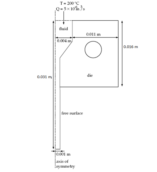
This tutorial examines the coupled problem of non-isothermal flow of a fluid and heat conduction in an axisymmetric steel die. As shown in Figure 3.1: Problem Description, the melt enters the domain at a fixed temperature, = 200°C and at a given flow rate, = 5 10⁻⁶m³/s. The problem involves flow, heat transfer by conduction and convection, and heat generation by viscous dissipation. Energy, momentum, and incompressibility equations are solved in the fluid domain. The energy equation for heat transport problems is solved in the solid (die) domain.

In solving for the free surface location, the position variables are also coupled to the temperature, velocity, and pressure fields. To solve the coupled problem, you will define two sub-tasks: one each for the fluid (sub-task 1) and the solid (sub-task 2). Each sub-task contains a particular model, domain of definition, material properties, and boundary conditions, including interface conditions with the other sub-task. The sub-tasks are coupled because the global solution of the problem depends on the values of the solution variables at the intersection of the fluid and solid domains.

Figure 3.1: Problem Description

The high flow rate introduces strong nonlinearity in the problem, which can lead to a loss of convergence in the iterative scheme. In Polyflow Classic, convergence strategies are available to solve such highly nonlinear problems.

The material properties of the generalized Newtonian fluid are:

	= density (950 kg/m³)
	= heat capacity per unit mass (2300 J/kg-°C)
	= thermal conductivity (0.5 W/m-°C)

Viscous heating is taken into account and the shear-rate dependence of viscosity obeys the Bird-Carreau law. For the solid region, the thermal conductivity () is 30 W/m-°C.

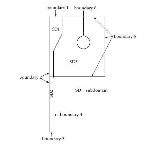
The boundary sets for the problem are shown in Figure 3.2: Boundaries and Subdomains, and the flow and thermal conditions for the fluid and the die at the boundaries of the domains are:

intersection of SUBDOMAIN_1 and SUBDOMAIN_3: interface
boundary 1: flow inlet (=200°C, = 5 × 10^-6 m³/s)
boundary 2: symmetry axis
boundary 3: insulated, zero force
boundary 4: free surface with convective heat transfer to surroundings ( = 20 W/m²-°C, _α= 20°C)
boundary 5: convective heat transfer to surroundings ( = 20 W/m²-°C, _α= 20°C)
boundary 6: convective heat transfer to surroundings ( = 20 W/m²-°C, _α= 20°C)

Figure 3.2: Boundaries and Subdomains

3.4. Setup and Solution

The following sections describe the setup and solution steps for this tutorial:

3.4.1. Preparation

To prepare for running this tutorial:

Prepare a working folder for your simulation.
Download the non_iso_flow.zip file here .
Unzip the non_iso_flow.zip file you have downloaded to your working folder.
The mesh file die.msh can be found in the unzipped folder.
Start Workbench from Start > Ansys 2025 R1 > Workbench 2025 R1.

3.4.2. Project and Mesh

Create a Fluid Flow (Polyflow Classic) analysis system by drag and drop in Workbench.
Save the Ansys Workbench project using File → Save, entering non-iso-flow as the name of the project.
Import the mesh file (die.msh).
Double-click the Setup cell to start Polydata.
When Polydata starts, the Create a new task menu item is highlighted, and the geometry for the problem is displayed in the Graphics Display window.

3.4.3. Create a Task for the Model

The flow problem for the generalized Newtonian fluid and the heat conduction problem in the solid are solved in two different sub-tasks. However, the task attributes are the same for both sub-tasks, so define a single task for the coupled problem.

Create a task for the model.
Create a new task
Select the following options:
- F.E.M. task
- 2D axisymmetric geometry
  The Current setup (above the selected options) is updated to reflect your selections. Since the problem involves an axisymmetric die, Polyflow Classic uses a 2D cylindrical reference frame (r,z) with r=0 as the axis of symmetry.
Click Accept the current setup.
The Create a sub-task menu item is highlighted.

3.4.4. Fluid Sub-Task 1

In the following steps you will define the flow problem, identify the domain of definition, set the relevant material properties for the fluid, and define boundary conditions along its boundaries.

Create a sub-task for the fluid.
Create a sub-task
1. Click Generalized Newtonian non-isothermal flow problem.
  Note: Be sure you are selecting the non-isothermal flow problem.
  A panel appears, asking for the title of the problem.
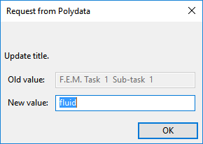
2. Enter fluid as the New value and click OK.
  The Domain of the sub-task menu item is highlighted.
Define the domain where the sub-task applies.
To solve the coupled problem, the computational domain is divided into three subdomains. There are two sub-tasks in this problem. Define a sub-task with its own model, material properties, and boundary conditions for the fluid region. Since this problem involves a free surface, the domain for sub-task 1 is divided into two subdomains: one for the region near the free surface (SUBDOMAIN_2) and the other for the rest of the fluid domain (SUBDOMAIN_1). In this problem, sub-task 1 applies to SUBDOMAIN_1 and SUBDOMAIN_2.
Domain of the sub-task
1. Select SUBDOMAIN_3 and click Remove.
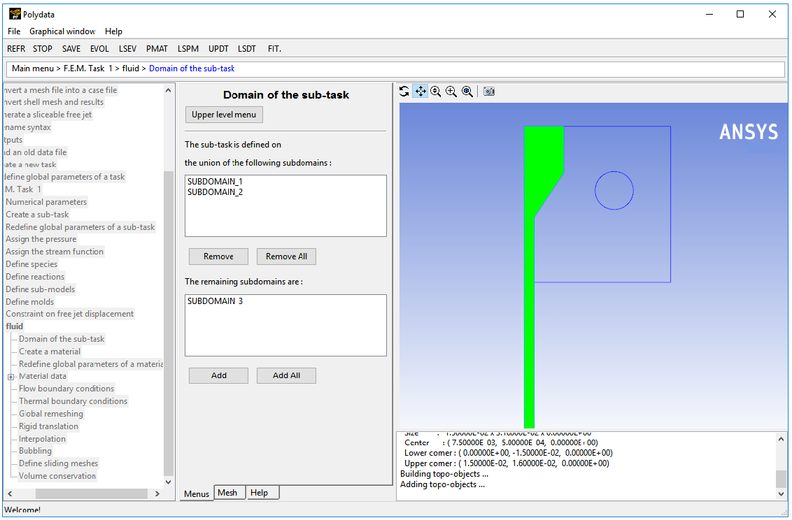
  SUBDOMAIN_3 is moved from the top list to the bottom list, indicating that subtask 1 is defined on SUBDOMAIN_1 and SUBDOMAIN_2.
2. Click Upper level menu at the top of the Domain of the sub-task menu.
  The Material data menu item is highlighted.
Specify the material properties for the fluid.
Polydata indicates the material properties that are relevant for your sub-task by graying out the irrelevant properties. In this sub-task, Polyflow Classic solves energy, incompressibility, and momentum equations. Hence, define viscosity, density, thermal conductivity, and heat capacity per unit mass. For a non-isothermal generalized Newtonian fluid, the viscosity depends on the shear rate and the temperature. Hence, define the shear-rate dependence of viscosity and the temperature dependence of viscosity.
Material data
1. Specify the shear-rate dependence of viscosity.
  Shear-rate dependence of viscosity
  1. Select Bird-Carreau law.
    Viscosity is defined by the Bird-Carreau law as
    (3–1)
    where is the viscosity at zero shear rate, is the shear rate, is the Bird-Carreau law index, and is the natural time.
  2. Specify the value , referred to as “fac” in the graphical user interface (compare the equation at the top of the Bird-Carreau law menu to Equation 3–1).
    Modify fac
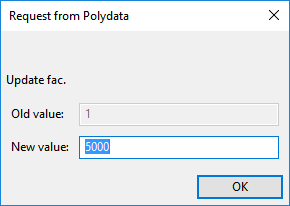
    Enter 5000 [units: Pa•s] as the New value and click OK.
  3. Specify the value , referred to as “tnat” in the graphical user interface.
    Modify tnat
    Enter 0.4 [units: s] as the New Value and click OK.
  4. Specify the value for , referred to as “expo” in the graphical user interface.
    Modify expo
    Enter 0.41 as the New Value and click OK.
  5. Click Upper level menu.
    When you click Upper level menu , Polydata displays the following warning message:
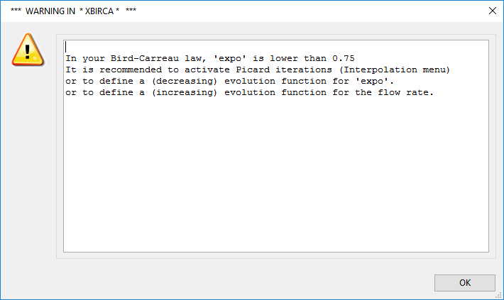
    For this tutorial, you will use the convergence strategy for viscosity/slip.
  6. Click OK to continue.
  7. Click Upper level menu again to continue with the Material Data specification.
2. Specify the temperature dependence of viscosity.
  Temperature dependence of viscosity
  For this problem, assume that the dependence of viscosity on temperature follows the Arrhenius law.
  1. Click Arrhenius law.
    The Arrhenius law is given as
    (3–2)
    where is the ratio of the activation energy to the thermodynamic constant and is a reference temperature for which = 1. The parameter denotes the absolute 0 temperature in your selected temperature scale. It is set to 0, when and are absolute temperatures. In this example, specify the temperatures in Celsius, so enter a value of -273 for .
  2. Specify the value for , referred to as “alfa” in the graphical user interface (compare the equation at the top of the Temperature dependence of viscosity menu to Equation 3–2).
    Modify alfa
    Enter 2300 [units: 1/°C] as the New Value and click OK.
  3. Specify the value for , referred to as “talfa” by the graphical user interface.
    Modify talfa
    Enter 200 [units: °C] as the New Value and click OK.
  4. Specify the value for , referred to as “t0” by the graphical user interface.
    Modify t0
    Enter -273 [units: °C] as the New Value and click OK.
  5. Click Upper level menu two times to continue with the Material Data specification.
3. Click Density.
  Specify a constant value for density.
  Modification of density
  1. Enter 950 [units: kg/m³] as the New value and click OK.
  2. Click Upper level menu to continue with the Material Data specification.
4. Click Thermal conductivity.
  Thermal conductivity is defined as a nonlinear function of the temperature:
  (3–3)
  For this problem, the thermal conductivity of the fluid is assumed to be a constant. So only the constant coefficient is modified.
  Modify a
  1. Enter 0.5 [units: W/m-°C] as the New Value and click OK.
  2. Click Upper level menu to continue with the Material Data specification.
5. Click Heat capacity per unit mass.
  The heat capacity per unit mass is defined as a nonlinear function of temperature:
  (3–4)
  The temperature variation of depends on the nature of the polymer melt. For this problem, is assumed to be constant, so only the constant coefficient is modified.
  Modify a
  1. Enter 2300 [units: J/kg-°C] as the New value and click OK.
  2. Click Upper level menu to continue with the Material Data specification.
6. Click Viscous (+ Wall friction) heating.
  When shearing occurs in a flow, the friction of the different fluid layers generates heat. When the fluid is highly viscous and/or the shear rate is high, the heating of the fluid caused by this phenomenon must be taken into account.
  1. Select Viscous + wall friction heating will be taken into account.
  2. Click Upper level menu to return to the Material Data specification.
7. Click Upper level menu to return to the fluid menu.
  The Flow boundary conditions menu item is highlighted.
Specify the flow boundary conditions for the fluid.
Flow boundary conditions
1. Retain the default condition Zero wall velocity (vn=vs=0) along SUBDOMAIN_3 at the intersection of SUBDOMAIN_1 and SUBDOMAIN_3.
  The liquid is assumed to stick to the wall, since at a solid-liquid interface the velocity of the liquid is that of the solid surface. This is known as the no-slip assumption because the liquid is assumed to adhere to the wall, and hence, has no velocity relative to the wall.
  By default, Polydata imposes = = 0 along all boundaries. No action is required to accept the default condition.
2. Set the conditions at the flow inlet (BOUNDARY_1).
  1. Select Zero wall velocity (vn=vs=0) along BOUNDARY_1 and click Modify.
  2. Click Inflow.
  3. Select Volumetric flow rate.
  4. Select Modify volumetric flow rate.
    Polydata prompts for the new value of the volumetric /mass flow rate.
    Enter 5e-06 [units: m³/s] as the New Value and click OK.
  5. Select Automatic option.
    When the Automatic option is selected, Polydata automatically chooses the most appropriate method to compute the inflow condition.
  6. Click Upper level menu to return to the Flow boundary conditions menu.
3. Retain the default condition, Axis of symmetry along BOUNDARY_2.
  For axisymmetric models, Polydata recognizes the axis of symmetry from the mesh file, and automatically imposes the symmetry condition along the line = 0. This condition imposes a zero surface normal velocity () and zero tangential force () along this boundary.
4. Set the conditions at the flow exit (BOUNDARY_3).
  It is assumed that a uniform velocity profile is reached at the exit. The melt is not subjected to any externally applied stress at the exit, so the condition of zero normal and tangential forces is selected.
  1. Select Zero wall velocity (vn=vs=0) along BOUNDARY_3 and click Modify.
  2. Click Normal and tangential forces imposed (fn, fs).
  3. Click Upper level menu to accept the default value of 0 [units: Pa] for .
  4. Click Upper level menu to accept the default value of 0 [units: Pa] for .
5. Set the conditions at the free surface (BOUNDARY_4).
  In a steady-state problem, the velocity field must be tangential to a free surface, since no fluid particles leave the domain through the free surface. This constraint is called the kinematic condition, = 0. This equation requires an initial condition, which is the starting line of the free surface. In this problem, the starting line of the free surface is the intersection of BOUNDARY_4 and SUBDOMAIN_3 (see Figure 3.2: Boundaries and Subdomains ).
  1. Select Zero wall velocity (vn=vs=0) along BOUNDARY_4 and click Modify.
  2. Click Free surface.
  3. Click Boundary conditions on the moving surface.
  4. Select No condition along SUBDOMAIN_3 and click Modify.
  5. Click Position imposed.
  6. Click Upper level menu.
  7. Click Upper level menu to return to the Kinematic condition menu.
  8. Click Upwinding in the kinematic equation.
  9. Click Direction of motion.
  10. Click No condition along whole surface and click Modify.
  11. Select Modify the constraint on the Y-component.
    Polydata prompts for the new value of the Y-component of the direction-of-displacement vector.
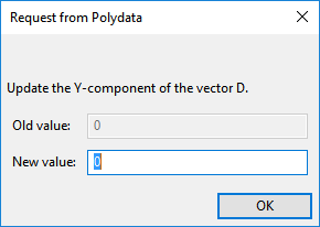
  12. Retain the default value of 0 and click OK.
  13. Click Accept the current condition.
  14. Click Upper level menu to return to the Kinematic condition menu.
  15. Click Upper level menu to return to the Flow boundary condition menu.
6. Click Upper level menu to return to the fluid menu.
Specify the thermal boundary conditions for the fluid.
For non-isothermal problems, specify either the temperature or the heat flux on each boundary set.
Thermal boundary conditions
1. Set the conditions at the intersection of SUBDOMAIN_1 and SUBDOMAIN_3.
  Set an interface condition at the intersection of SUBDOMAIN_1 and SUBDOMAIN_3. This condition ensures the continuity of the temperature field and the heat flux along the interface. Since the problem is coupled, the condition of continuity is essential for the global solution of the temperature and heat flux variables.
  1. Select Temperature imposed along SUBDOMAIN_3 and click Modify.
  2. Click Interface.
  3. Click Upper level menu to accept the default setting (continuous heat flux along the interface).
    For an interface condition, both the heat flux and temperature are usually continuous along the interface. It is possible to specify a nonzero value for the heat flux jump (), but this is mainly used in problems where internal radiation is simulated. Accept the default value for the definition of heat flux discontinuity (=0).
2. Set the condition at the flow inlet (BOUNDARY_1).
  1. Select Temperature imposed along BOUNDARY_1 and click Modify.
  2. Click Temperature imposed.
  3. Select Constant.
    Polydata prompts for the value of the temperature.
  4. Enter 200 [units: °C] as the New Value and click OK.
  5. Click Upper level menu to return to the Thermal boundary conditions menu.
3. Retain the default condition, Axis of symmetry along BOUNDARY_2.
4. Set the conditions at the flow exit (BOUNDARY_3).
  1. Select Temperature imposed along BOUNDARY_3 and click Modify.
  2. Click Insulated boundary/symmetry.
5. Set the conditions at the free surface (BOUNDARY_4)
  1. Select Temperature imposed along BOUNDARY_4 and click Modify.
  2. Click Flux density imposed.
    If the heat transfer from radiation is neglected, the heat flux can be written as
    
    (3–5)
    
    where is the heat convection coefficient and is the reference temperature (in this case, the temperature of the air surrounding the extrudate).
  3. Specify the value of .
    Modify alpha
    Enter 20 [units: W/m²-°C] as the New value and click OK.
  4. Specify the value of .
    Modify Talpha
    Enter 20 [units: °C] as the New value and click OK.
  5. Click Upper level menu to return to the Thermal boundary conditions menu.
6. Click Upper level menu to return to the fluid menu.
  The Global remeshing menu item is highlighted.
Define remeshing for SUBDOMAIN_2.
This model involves a free surface for which the position is unknown. A portion of the mesh is affected by the relocation of this boundary. Hence, a remeshing technique is applied on this part of the mesh. The free surface is entirely contained within SUBDOMAIN_2 and hence, only SUBDOMAIN_2 is affected by the relocation of the free surface.
Global remeshing
1. Specify the region where the remeshing is to be performed (SUBDOMAIN_2).
  1-st local remeshing
  1. Select SUBDOMAIN_1 and click Remove.
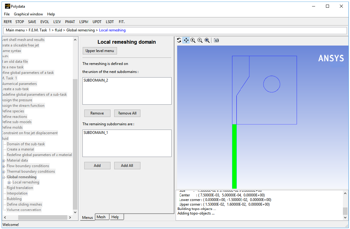
    SUBDOMAIN_1 is moved from the top list to the bottom list, indicating that only SUBDOMAIN_2 will be remeshed.
  2. Click Upper level menu.
    The Method of spines menu item is highlighted.
2. Define the parameters for the system of spines.
  The purpose of the remeshing technique is to relocate internal nodes according to the displacement of boundary nodes due to the motion of the free surface. Mesh nodes are organized along lines of remeshing (spines), which are collections of nodes logically arranged in a one-dimensional manner.
  Polydata requires the specification of the first and last spines (inlet and outlet) that the fluid encounters. In this case, the inlet of spines is the intersection of SUBDOMAIN_2 with SUBDOMAIN_1, and the outlet of spines is the intersection of SUBDOMAIN_2 with the flow exit (BOUNDARY_3).
  Method of Spines
  1. Specify the inlet for the system of spines by selecting SUBDOMAIN_1 and clicking Modify.
    1. Select Part of inlet section.
    2. Select Upper level menu.
  2. Specify the outlet for the system of spines by selecting BOUNDARY_3 and clicking Modify.
    1. Select Part of outlet section.
    2. Select Upper level menu.
  3. Click Accept the current setup in the Element distortion check menu.
    The finite-element mesh can undergo great deformations. The Element distortion check menu deals with the detection of all possible distortions of the elements.
    For this problem, accept the default options and proceed to the next step.
3. Click Upper level menu to return to the fluid menu.
Select a suitable discretization scheme to increase the accuracy of the calculation.
Interpolation
You can expect important temperature gradients in the calculation. Therefore, you can retain the quadratic interpolation (9 unknowns per element) for velocity and the linear interpolation (4 unknowns per element) for pressure, but it is recommended that you select the 4x4 interpolation for temperature. In the 4x4 discretization scheme, each finite element is divided into 16 sub-elements, with the temperature being linearly interpolated over each sub-element. This leads to 25 temperature unknowns per element.
1. Scroll down to select 4x4 element for temperature in the Interpolation menu.
  The Current setup (at the top of the menu) is updated to reflect your selection.
2. Click Upper level menu two times to return to the F.E.M. Task 1 menu.

3.4.5. Die Sub-Task

In the following steps you will define the heat conduction problem, identify the domain of definition, set the relevant material properties for the die, and define the boundary conditions along its boundaries.

Create a sub-task for the die.
Create a sub-task
1. Polydata warns you that a thermal interface has been defined, and that no other sub-task shares the interface. Click OK to close the warning.
2. Polydata asks if you want to copy data from an existing sub-task.
3. Click No, since this sub-task has different parameters associated with it.
4. Select Heat conduction problem.
  A panel appears, asking for the title of the problem.
5. Enter solid as the New Value and click OK.
  The Domain of the sub-task menu item is highlighted.
Define the domain where the sub-task applies (SUBDOMAIN_3).
Domain of the sub-task
1. Select SUBDOMAIN_1 and click Remove.
2. Select SUBDOMAIN_2 and click Remove.
3. Click Upper level menu at the top of the Domain of the sub-task menu.
  The Material data menu item is highlighted.
Specify the material properties for the die.
For this problem, specify a constant value for the thermal conductivity .
Material data
1. Select Thermal conductivity.
  For this problem, thermal conductivity is assumed to be a constant, so only the constant coefficient is modified.
2. Select Modify a.
3. Enter 30 [units: W/m-°C] as the New value and click OK.
4. Click Upper level menu two times to return to the solid menu.
  The Thermal boundary conditions menu item is highlighted.
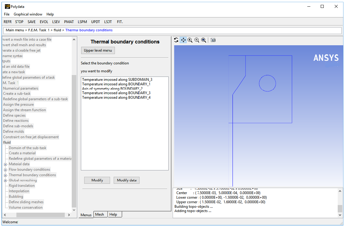
Specify the thermal boundary conditions for the die.
Set the conditions at each of the boundaries of the domain. The selected boundary set will be highlighted (in red) in the graphics window as you select them..
Thermal boundary conditions
1. Set the conditions at the intersection of SUBDOMAIN_1 and SUBDOMAIN_3.
  Set an interface condition at the intersection of the subdomains.
  1. Select Temperature imposed along SUBDOMAIN_1 and click Modify.
  2. Click Interface.
  3. Click Upper level menu to accept the default option for continuity of temperature and heat flux.
2. Set the conditions on the outer boundary of the die (BOUNDARY_5).
  1. Select Temperature imposed along BOUNDARY_5 and click Modify.
  2. Click Flux density imposed.
    Take only the heat convection into account: see Equation 3–5 .
  3. Specify the value of .
    Modifiy alpha
    Enter 20 [units: W/m²-°C] as the New Value and click OK.
  4. Specify the value of .
    Modifiy Talpha
    Enter 20 [units: °C] as the New Value and click OK.
  5. Click Upper level menu to return to the Thermal boundary conditions menu.
3. Set the conditions at the inner boundary of the die (BOUNDARY_6).
  1. Select Temperature imposed along BOUNDARY_6 and click Modify.
  2. Select Flux density imposed.
  3. Specify the value of .
    Modify alpha
    Enter 20 [units: W/m²-°C] as the New value and click OK.
  4. Specify the value of .
    Modifiy Talpha
    Enter 20 [units: °C] as the New Value and click OK.
  5. Click Upper level menu to return to the Thermal boundary conditions menu.
Click Upper level menu twice to return to the F.E.M. Task 1 menu.

3.4.6. Outputs

Outputs

Set the system of units to output to CFD-Post.
Set units for CFD-Post, Ansys Mapper or Iges
1. Modify the current system of units.
  Modify system of Units
2. Specify the new system of units.
  Set to metric_MKSA+Celsius
Click Upper level menu three times to return to the top-level Polydata menu.

3.4.7. Save and Exit Polydata

Save and exit

Select Enable convergence strategy for rheology / slip in the Convergence strategies menu, and click Accept.
Click Accept in the Field Management menu.
This confirms that the default Current field(s) are correct.
Click Continue.
This accepts the default names for graphical output files (cfx.res) that are to be saved for postprocessing, and for the Polyflow Classic format results file (res).

3.4.8. Solution

Run Polyflow Classic to calculate a solution for the model you just defined using Polydata.

Run Polyflow Classic by right-clicking the Solution cell of the simulation and selecting Update.
This executes Polyflow Classic using the data file as standard input, and writes information about the problem description, calculations, and convergence to a listing file (polyflow.lst).
Check for convergence in the listing file.
1. Right-click the Solution cell and select Listing Viewer....
  Workbench opens the View listing file panel, which displays the listing file.
2. It is a common practice to confirm that the solution proceeded as expected by looking for the following printed at the bottom of the listing file:
```
The computation succeeded.
```

3.4.9. Postprocessing

Use CFD-Post to view the results of the Polyflow Classic simulation.

Double-click the Results cell in the Workbench analysis and read the results files saved by Polyflow Classic.
CFD-Post reads the solution fields that were saved to the results file.
Align the view.
In the graphical window, right-click, and select the option Predefined Camera.
1. Right-click in the graphical window and select View from +Z under Predefined Camera.
2. To remove the ruler right-click in the graphical window, select Viewer Options, and disable Ruler Visibility.
Display contours of pressure in the fluid region (SUBDOMAIN_1 and SUBDOMAIN_2).
1. Click the Insert menu and select Contour or click the button.
2. In the panel that opens, click OK to accept the default name (Contour 1) display the details view below the Outline tab.
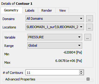
3. Perform the following steps In the Geometry tab of the details view for Contour 1:
  1. Next to Locations, click the ellipsis button ( ) on the right and select SUBDOMAIN_1_surf and SUBDOMAIN_2_surf (use Ctrl to select multiple items).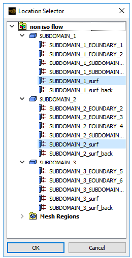
    Click OK to close the Location Selector dialog box.
  2. Select PRESSURE from the Variable drop-down list, or click the ellipsis button ( ) on the right and select PRESSURE.
  3. Click Apply.
Figure 3.3: Contours of Pressure
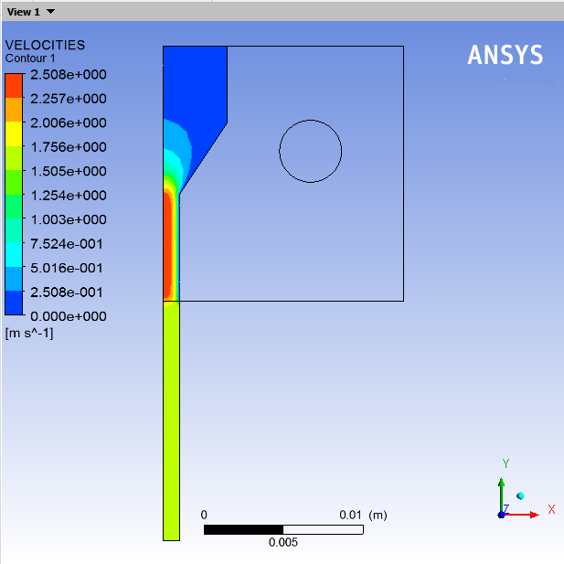
Display contours of velocity in the fluid region.
1. In the details view of Contour 1, select VELOCITIES from the Variable drop-down list.
2. Click Apply.
Figure 3.4: Velocity Profile

The fluid experiences high velocity gradients in the narrow section of the die. This leads to important viscous dissipation effects that cause the temperature of the melt to increase.
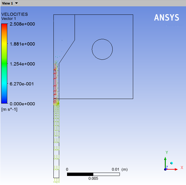
Display velocity vectors for the two fluid subdomains.
1. In the Outline tab under User Locations and Plots, disable Contour 1.
2. Click the Insert menu and select Vector or click the button.
3. Click OK to accept the default name (Vector 1) and open the details view below the Outline tab.
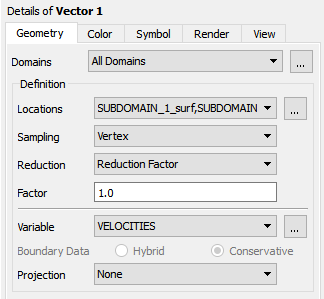
4. Perform the following steps in the details view of Vector 1:
  1. In the Geometry tab, click the button next to Locations to open the Location Selector dialog box.
  2. Select SUBDOMAIN_1_surf and SUBDOMAIN_2_surf (use Ctrl to select multiple items).
    Click OK to close the Location Selector dialog box.
  3. In the Symbol tab, select Arrow3D and retain the default Symbol Size of 1.0.
  4. Click Apply.
Figure 3.5: Velocity Vectors

The velocity vectors in the wide section of the die are very small compared to those in the narrow section of the die (Figure 3.5: Velocity Vectors). Also, the important velocity re-arrangement takes place at the die exit. This leads to the swelling of the extrudate.
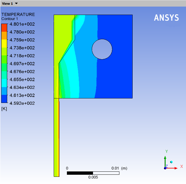
Display the temperature distribution in the solid and the fluid regions.
1. In the Outline tab, under User Locations and Plots, disable Vector 1, and enable and double-click Contour 1.
2. In the details of Contour 1, define the temperature contours.
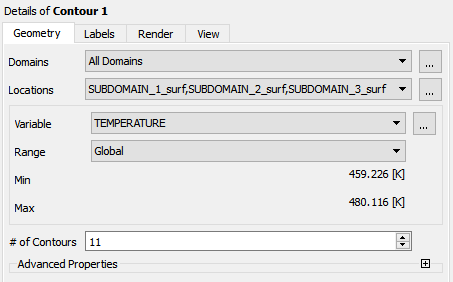
  1. Next to Locations, click the ellipsis button ( ) on the right and select SUBDOMAIN_1_surf, SUBDOMAIN_2_surf and SUBDOMAIN_3_surf (use Ctrl to select multiple items).
    Click OK to close the Location Selector dialog box.
  2. Select TEMPERATURE from the Variable drop-down list.
  3. Click Apply.
Figure 3.6: Temperature Profile

Figure 3.7: Temperature Profile Near the Die Exit

Figure 3.7: Temperature Profile Near the Die Exit shows a magnified view of the temperature contours near the die exit. The high velocity gradients near the die exit lead to an important viscous dissipation effect. The temperature of the polymer melt increases from the converging zone to the die lip. This increase in temperature must be monitored to avoid melt degradation. The simulation helps optimize the geometry of the die, the flow section for the cooling fluid, and other conditions in order to maximize the flow rate and the extrudate speed.
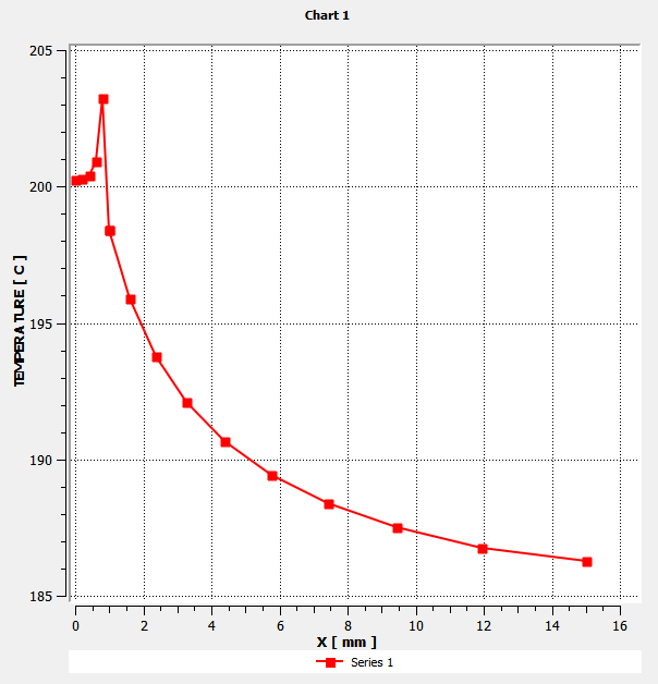
Create a 2D plot on a cross-section of the die.
1. Verify that you have millimeters selected as your units for length in CFD-Post.
  Edit → Options... → Units
2. Define the line for the plot with the points (0, 1, 0) and (15, 1, 0).
  1. Select Line from the Location menu ( ).
  2. Click OK to accept the default name (Line 1) and display the details view below the Outline tab.
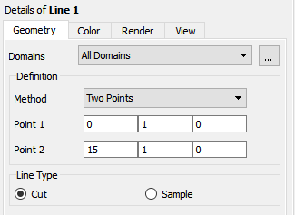
  3. Enter 0, 1, 0 for Point 1 and 15, 1, 0 for Point 2.
  4. Select the Cut option button under Line Type.
  5. Click Apply.
3. Create a plot.
  1. Click the chart button .
  2. Click OK to accept the default name (Chart 1) and display the details view below the Outline tab.
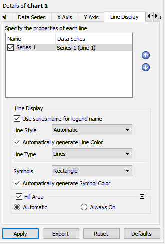
  3. In the General tab of the details view, ensure XY is selected for the chart Type and disable Display Title.
  4. In the Data Series tab, select Line 1 from the Locations drop-down list for Series 1.
  5. In the X Axis tab, select X from the Variable drop-down list.
  6. In the Y Axis tab, select TEMPERATURE from the Variable drop-down list.
  7. With Series 1 (Line 1) enabled under the Line Display tab, select Rectangle from the Symbols drop-down list. Retain the default setting forAutomatically generate Symbol Color.
  8. Click Apply.
Figure 3.8: Temperature Profile Across the Die

3.5. Summary

In this tutorial, you solved the non-isothermal flow of a polymer melt through a cooled die. You set the material properties for the melt and supplied suitable boundary conditions. A specific interpolation scheme was used for the temperature in order to cope with the important gradients.