Chapter 7: Flow of Two Immiscible Fluids

This tutorial is divided into the following sections:

7.1. Introduction

This tutorial examines the flow of two fluids in a single die. Two polymer melts with distinct physical properties are fed through different channels into a die. The aim of the calculation is to predict the location of the interface between the two fluids.

In this tutorial you will learn how to:

Define a moving interface problem.
Create multiple sub-tasks.
Set material properties and boundary conditions for a moving interface problem.
Select a remeshing method.

7.2. Prerequisites

This tutorial assumes that you are familiar with the menu structure in Polydata and Workbench and that you have solved or read 2.5D Axisymmetric Extrusion. Some steps in the set up procedure will not be shown explicitly.

7.3. Problem Description

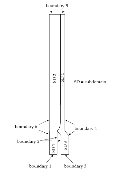
This problem analyzes the flow of two immiscible Newtonian fluids (fluid 1 and fluid 2) through a die of diameter 1 cm, as shown in Figure 7.1: A Schematic Diagram of the Two Fluids in the Die. The melts are fed into the die through boundaries 1 and 3 (see Figure 7.2: Boundary Sets and Subdomains for the Problem). The flow rates for the two fluids are not equal. The fluids come into contact in the die, creating an interface. The location of the interface is unknown and will be determined by Polyflow Classic. The location of the interface depends on the physical properties of the fluids, the flow rates of the fluids, and the geometry of the die.

Incompressibility and momentum equations are solved in the fluid domains. To solve the fully coupled problem, two sub-tasks are defined one each for fluid 1 (sub-task 1) and fluid 2 (sub-task 2). Each sub-task will contain a particular model, domain of definition, material properties, and boundary conditions, including the moving interface along the intersection of the two sub-tasks.

The domain of definition for the problem is divided into four subdomains: sub-task 1 is defined on subdomain 1 and subdomain 2, and sub-task 2 is defined on subdomain 3 and subdomain 4 (see Figure 7.2: Boundary Sets and Subdomains for the Problem). Each sub-task is defined over two subdomains to allow for the definition of the remeshing method only where it is necessary, (in the area near the moving interface).

Fluid 1 has a viscosity of = 10000 poise, and fluid 2 has a viscosity of = 5000 poise.

Figure 7.1: A Schematic Diagram of the Two Fluids in the Die

The boundary sets for the problem are shown in Figure 7.2: Boundary Sets and Subdomains for the Problem.

Figure 7.2: Boundary Sets and Subdomains for the Problem

The conditions at the boundaries of the domains are:

boundary 1: flow inlet for fluid 1, volumetric flow rate = 3 cm³/s
boundary 2: outer wall common to subdomain 1 and subdomain 3: zero velocity
boundary 3: flow inlet for fluid 2, volumetric flow rate = 1 cm³/s
boundary 4: outer wall common to subdomain 3 and subdomain 4: zero velocity
boundary 5: flow exit for both fluids
boundary 6: outer wall common to subdomain 1 and subdomain 2: zero velocity

An interface is defined at the intersection of subdomain 2 and subdomain 4. In this problem, the interface is a moving one, since the exact line of separation between the fluids is unknown.

7.4. Setup and Solution

The following sections describe the setup and solution steps for this tutorial:

7.4.1. Preparation

To prepare for running this tutorial:

Prepare a working folder for your simulation.
Download the two_fluids.zip file here .
Unzip the two_fluids.zip file you have downloaded to your working folder.
The mesh file fluids.msh can be found in the unzipped folder.
Start Workbench from Start > Ansys 2025 R1 > Workbench 2025 R1.

7.4.2. Project and Mesh

Create a Fluid Flow (Polyflow Classic) analysis system by drag and drop in Workbench.
Save the Ansys Workbench project using File → Save, entering two-fluids as the name of the project.
Import the mesh file (fluids.msh).
Double-click the Setup cell to start Polydata.
When Polydata starts, the Create a new task menu item is highlighted, and the geometry for the problem is displayed in the Graphics Display window.

7.4.3. Create a Task for the Model

In the following steps you will define a single task that represents the global problem. Since this tutorial deals with two fluids, each with its own physical properties, you will need to define two different sub-tasks (one for each fluid) in subsequent sections.

Create a task for the model.

Create a new task

Select the following options:
- F.E.M. task
- Steady-state problem(s)
- 2D axisymmetric geometry
Click Accept the current setup.
The Create a sub-task menu item is highlighted.

7.4.4. Fluid 1 Sub-Task

In the following steps you will define the nature of the flow problem, identify the domain of definition, set the relevant material properties for fluid 1, and define boundary conditions along its boundaries.

Create a sub-task for fluid 1.
Create a sub-task
1. Click Generalized Newtonian isothermal flow problem.
  A small dialog box appears asking for the title of the problem.
2. Enter fluid 1 as the New value and click OK.
  The Domain of the sub-task menu item is highlighted.
Define the domain where the sub-task applies.
Sub-task 1 is defined for SUBDOMAIN2 (the region of fluid 1 near the moving interface) and SUBDOMAIN1 (the rest of fluid 1), as shown in Figure 7.2: Boundary Sets and Subdomains for the Problem.
Domain of the sub-task
1. Select SUBDOMAIN3 and click Remove.
2. Select SUBDOMAIN4 and click Remove.
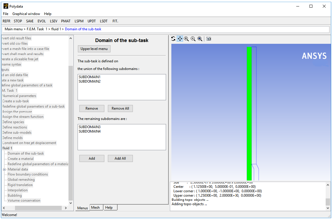
3. Click Upper level menu.
  The Material data menu item is highlighted.
Specify the material data properties for fluid 1.
Material Data
Polydata indicates which material properties are relevant for your sub-task by graying out the irrelevant properties. In this case, viscosity, density, inertia terms, and gravity are available for specification. For this model, define only the viscosity of the material.
Click Shear-rate dependence of viscosity.
Click Constant viscosity.
Specify the value for , referred to as “fac” in the graphical user interface.
Modify fac
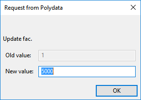
Polydata prompts for a new value of .
Enter 10000 [units: poise] as the New value and click OK.
Click Upper level menu three times to return to the fluid 1 menu.
The Flow boundary conditions menu item is highlighted.
Specify the flow boundary conditions for fluid 1 (SUBDOMAIN1 and SUBDOMAIN2).
Flow boundary conditions
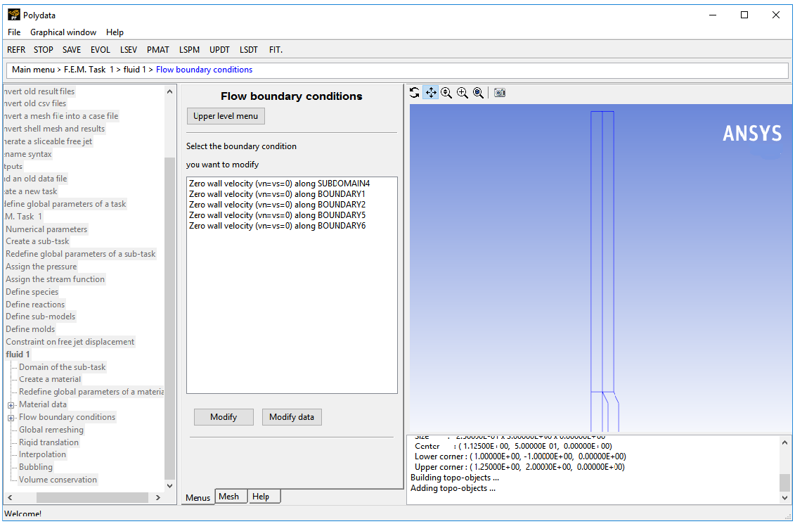
1. Set the conditions along the intersection of SUBDOMAIN2 and SUBDOMAIN4.
  The boundary uses the interface condition, which is the standard boundary condition between two adjacent fluids. This condition establishes the continuity of the velocity field and the contact forces in the momentum equation.
  The position of the line separating the two fluids is unknown at the start of the problem and is calculated as part of the solution, so the intersection will be defined as a moving interface. In steady flows and problems involving immiscible fluids, the interface must be a streamline. To satisfy this condition and to obtain the exact location of the line of separation, an additional equation, the kinematic condition, ( = 0), is added to the system. This guarantees that the material points do not cross the interface.
  1. Select Zero wall velocity (vn=vs=0) along SUBDOMAIN4 and click Modify.
  2. Click Interface.
  3. Select Switch to moving interface.
  4. Click Specify moving interface parameters.
  5. Click Boundary conditions on the moving surface.
    Polydata asks you to select the boundary or subdomain on which the position of the moving surface is to be imposed.
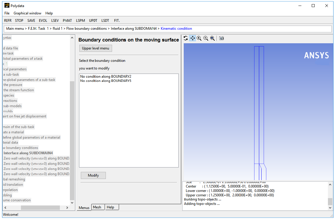
  6. Select No condition along BOUNDARY2 and click Modify.
  7. Select Position imposed.
  8. Click Upper level menu twice to return to the Kinematic condition menu.
  9. Select Upwinding in the kinematic equation. Click Upper level menu.
  10. Click Accept the current setup to return to the Flow boundary conditions menu.
2. Set the conditions at the flow inlet for fluid 1 (BOUNDARY1).
  1. Select Zero wall velocity (vn=vs=0) along BOUNDARY1 and click Modify.
  2. Click Inflow.
  3. Click Modify volumetric flow rate.
    Polydata prompts you for the volumetric flow rate.
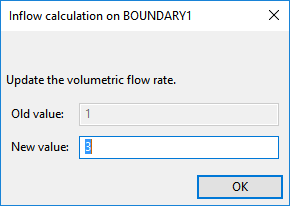
  4. Enter 3 [units: cm³/s] as the New value and click OK.
  5. Ensure Automatic is selected and click Upper level menu.
    When this option is selected, Polydata automatically chooses the most appropriate method to compute the inflow condition.
  6. Retain the default condition Zero wall velocity (vn=vs=0) along BOUNDARY2 at the outer wall of SUBDOMAIN1 (BOUNDARY2).
    At a solid-liquid interface, the velocity of the liquid is that of the solid surface. Hence the fluid is assumed to stick to the wall. This is known as the no-slip assumption because the liquid is assumed to adhere to the wall, and therefore has no velocity relative to the wall.
    By default, Polydata imposes Zero wall velocity ( = = 0) along all boundaries.
3. Set the conditions at the flow outlet (BOUNDARY5).
  It is assumed that a fully developed velocity profile is reached at the exit, so the outflow condition is appropriate. This condition essentially imposes a zero normal force () that includes a pressure term, and zero tangential velocity ().
  1. Select Zero wall velocity (vn=vs=0) along BOUNDARY5 and click Modify.
  2. Click Outflow.
4. Retain the default condition Zero wall velocity (vn=vs=0) along BOUNDARY6 at the outer wall common to SUBDOMAIN1 and SUBDOMAIN2 (BOUNDARY6).
  The fluid is assumed to stick to the wall, since at a solid-liquid interface the velocity of the liquid is that of the solid surface.
5. Click Upper level menu to return to the fluid 1 menu.
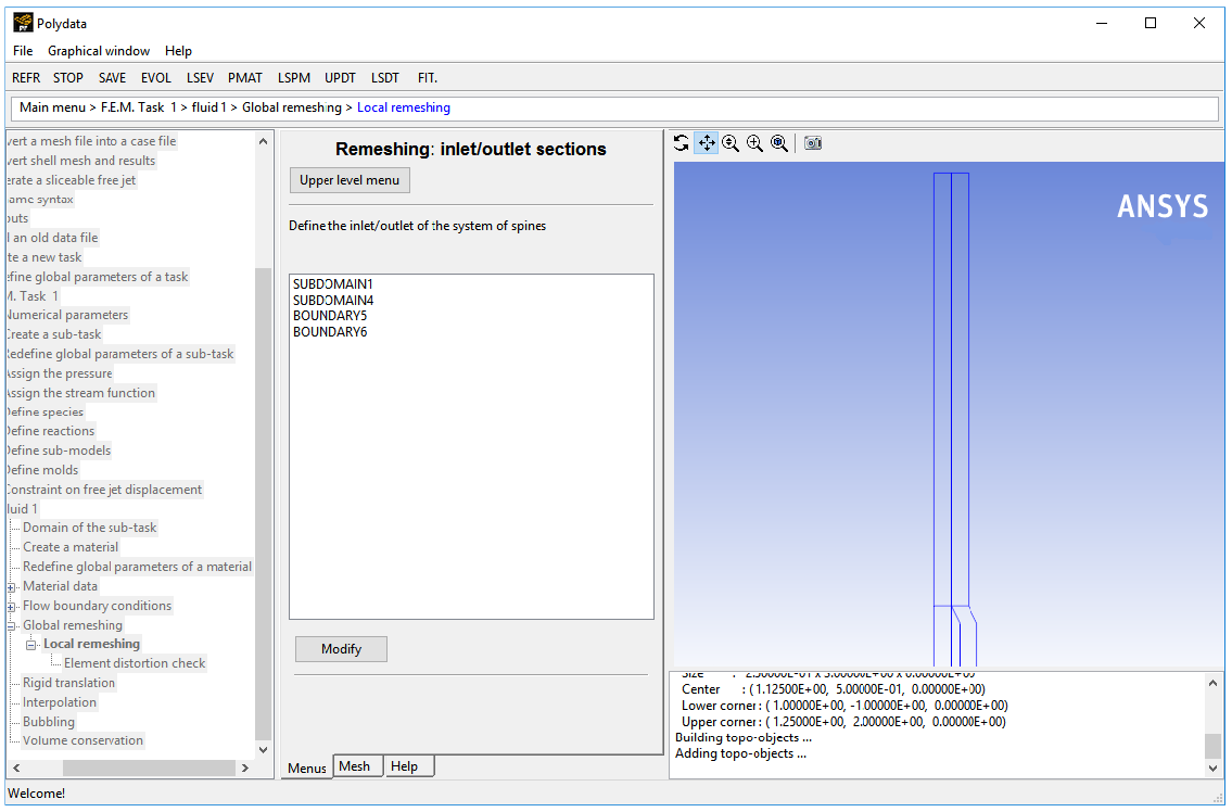
Define remeshing for SUBDOMAIN2.
This model involves a free surface, whose shape is unknown a priori, which will be calculated together with the flow equations. A portion of the mesh is affected by the relocation of this boundary. Hence a remeshing technique is applied on this part of the mesh. The moving interface is entirely contained within SUBDOMAIN2, and hence only SUBDOMAIN2 will be affected by the relocation of the moving interface.
Global remeshing
1. Specify the region where the remeshing is to be performed (SUBDOMAIN2).
  If you have a complex geometry, it may be necessary to split it into additional subdomains in order to define a specific remeshing method on each of them.
  For this purpose, Polydata allows you to create several local remeshings. For this problem, a single local remeshing is sufficient.
  1–st local remeshing
  1. Select SUBDOMAIN1 and click Remove.
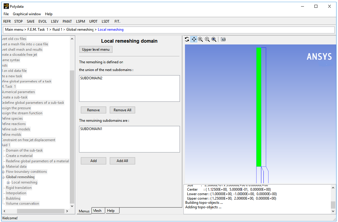
  2. Click Upper level menu.
    The Method of Spines menu item is highlighted.
2. Define the parameters for the system of spines.
  The purpose of the remeshing technique is to relocate internal nodes according to the displacement of boundary nodes due to the motion of the interface. Mesh nodes must be organized along lines of remeshing (spines), which are collections of nodes logically arranged in a one-dimensional manner. Polydata requires the specification of the first and last spines that the fluid encounters (inlet of spines and outlet of spines, respectively). In this case, the inlet of spines is the intersection of SUBDOMAIN2 with SUBDOMAIN1, and the outlet of spines is the intersection of SUBDOMAIN2 with the flow exit (BOUNDARY5).
  Method of Spines
  1. To specify the inlet for the system of spines, select SUBDOMAIN1 and click Modify.
    1. Select Part of inlet section.
    2. Select Upper level menu.
  2. Specify the outlet for the system of spines, select BOUNDARY5 and click Modify.
    1. Select Part of outlet section.
    2. Select Upper level menu.
  3. Click Upper level menu two times.
    The F.E.M. Task 1 menu is displayed.

7.4.5. Fluid 2 Sub-Task

In the following steps you will define the nature of the flow problem, identify the domain of definition, set the relevant material properties for fluid 2, and define the boundary conditions along its boundaries.

Create a sub-task for fluid 2.
Create a sub-task
1. Polydata asks you if you want to copy data from an existing sub-task.
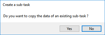
2. Click No, since this sub-task has different parameters associated with it.
3. Click Generalized Newtonian isothermal flow problem.
  A small dialog box appears asking for the title of the problem.
4. Enter fluid 2 as the New value and click OK.
  The Domain of the sub-task menu item is highlighted.
Define the domain where the sub-task applies.
Domain of the sub-task
1. Select SUBDOMAIN1 and click Remove.
2. Select SUBDOMAIN2 and click Remove.
3. Click Upper level menu.
  The Material data menu item is highlighted.
Specify the material data properties for fluid 2.
Material Data
For this model, define only the viscosity of the material.
1. Click Shear-rate dependence of viscosity.
2. Click Constant viscosity.
3. Specify the value for , referred to as “fac” in the graphical user interface.
  Modify fac
  Polydata prompts for a new value of .
  Enter 5000 [units: poise] as the New value and click OK.
4. Click Upper level menu three times to return to the fluid 2 menu.
  The Flow boundary conditions menu item is highlighted.
Specify the flow boundary conditions for fluid 2 (SUBDOMAIN3 and SUBDOMAIN4).
Flow boundary conditions
1. Set the conditions along the intersection of SUBDOMAIN2 and SUBDOMAIN4.
  1. Select Zero wall velocity (vn=vs=0) along SUBDOMAIN2 and click Modify.
  2. Click Interface.
    The interface condition was defined as a moving interface when setting the boundary conditions for fluid 1. So further inputs are not required to define the moving interface for fluid 2. Surface tension effects are neglected in this problem.
  3. Click Accept the current setup.
2. Retain the default condition Zero wall velocity (vn=vs=0) along BOUNDARY2 at the outer wall of SUBDOMAIN3 (BOUNDARY2).
3. Set the conditions at the flow inlet for fluid 2 (BOUNDARY3).
  1. Select Zero wall velocity (vn=vs=0) along BOUNDARY3 and click Modify.
  2. Click Inflow.
  3. Click Modify volumetric flow rate.
    Polydata prompts you for the volumetric flow rate.
  4. Accept the default value of 1 [units: cm³/s] for the flow rate by clicking OK.
  5. Ensure Automatic is selected, and click Upper level menu.
4. Retain the default condition Zero wall velocity (vn=vs=0) along BOUNDARY4 at the outer wall common to SUBDOMAIN3 and SUBDOMAIN4 (BOUNDARY4).
5. Set the conditions at the flow outlet for fluid 2 (BOUNDARY5).
  1. Select Zero wall velocity (vn=vs=0) along BOUNDARY5 and click Modify.
  2. Click Outflow.
6. Click Upper level menu to return to the Flow boundary conditions menu.
  The Global remeshing menu item is highlighted.
Define remeshing for SUBDOMAIN4.
Global remeshing
1. Specify the region where the remeshing is to be performed (SUBDOMAIN4).
  1–st local remeshing
  1. Select SUBDOMAIN3 and click Remove.
  2. Click Upper level menu.
    The Method of Spines menu item is highlighted.
2. Define the parameters for the system of spines.
  In this case, the inlet of spines is the intersection of SUBDOMAIN3 with SUBDOMAIN4, and the outlet of spines is the intersection of SUBDOMAIN4 with the flow exit (BOUNDARY5).
  Method of Spines
  1. Specify the inlet for the system of spines by selecting SUBDOMAIN3 and click Modify.
    1. Select Part of inlet section.
    2. Select Upper level menu.
  2. Specify the outlet for the system of spines by selecting BOUNDARY5 and click Modify.
    1. Select Part of outlet section.
    2. Select Upper level menu.
3. Click Upper level menu three times.
  The top-level Polydata menu is displayed.

7.4.6. Save and Exit Polydata

Save and exit

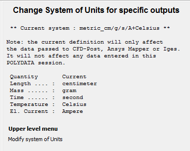
Polydata asks you to confirm the current system units and fields that are to be saved to the results file for postprocessing.

Specify the system of units for the simulation.
1. Click Modify system of units.
2. Select Set to metric_cm/g/s/A+Celsius.
3. Click Upper level menu twice.
Click Accept current setup in the Convergence strategies menu.
Click Accept in the Field Management menu.
This confirms that the default Current field(s) are correct.
Click Continue.
This accepts the default names for graphical output files (cfx.res) that are to be saved for postprocessing, and for the Polyflow Classic format results file (res).

7.4.7. Solution

Run Polyflow Classic to calculate a solution for the model you just defined using Polydata.

Run Polyflow Classic by right-clicking the Solution cell of the simulation and selecting Update.
This executes Polyflow Classic using the data file as standard input, and writes information about the problem description, calculations, and convergence to a listing file (polyflow.lst).
Check for convergence in the listing file.
1. Right-click the Solution cell and select Listing Viewer....
  Workbench opens the View listing file dialog box, which displays the listing file.
2. It is a common practice to confirm that the solution proceeded as expected by looking for the following printed at the bottom of the listing file:
```
The computation succeeded.
```

7.4.8. Postprocessing

Use CFD-Post to view the results of the Polyflow Classic simulation.

Double-click the Results tab in the Workbench analysis and read the results files saved by Polyflow Classic.
CFD-Post reads the solution fields that were saved to the results file.
Align the view.
1. In the graphical window, right-click, and select the option Predefined Camera.
2. Select View from +Z.
Display contours of velocity magnitude.
1. Click the Insert menu and select Contour or click the button.
2. Click OK to accept the default name (Contour 1) and display the details view below the Outline tab.
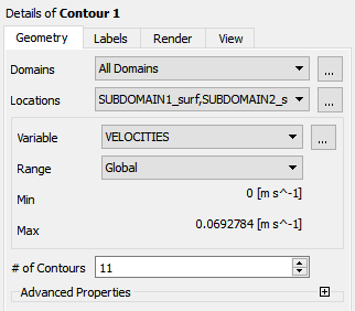
3. Perform the following steps in the details view:
  1. In the Geometry tab, click the button next to Locations.
  2. In the Location Selector dialog box that opens, select SUBDOMAIN1_surf, SUBDOMAIN2_surf, SUBDOMAIN3_surf, and SUBDOMAIN4_surf (use Ctrl for multiple selection) and then click OK.
  3. Select VELOCITIES from the Variable drop-down list (or by clicking ).
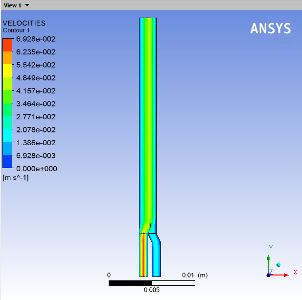
  4. Click Apply.
Figure 7.3: Contours of Velocity Magnitude

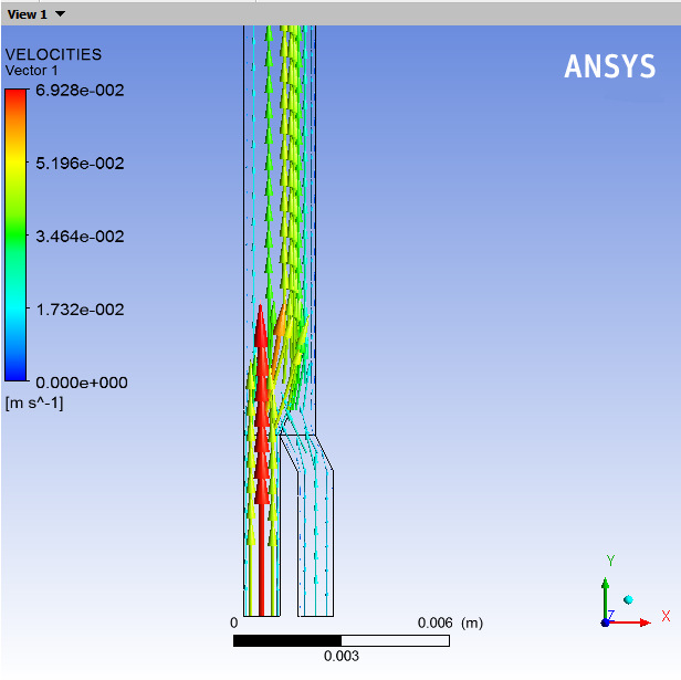
The velocity is much larger at the inlet of fluid 1 than at the inlet of fluid 2. There are two reasons for this:
- The flow rate is three times larger for fluid 1 than for fluid 2.
- You are modeling an annular die. Hence the flow section is smaller for the interior channel than for the exterior channel.
When the two fluids come into contact with each other, the interface between the two fluids is pushed towards the exterior of the annular die.
There are three reasons for this:
- The flow rate for fluid 1 is higher than for fluid 2.
- The die is annular, so even identical flow rates cause the interface to move in order to equilibrate the flow sections.
- The viscosity of fluid 1 is higher than the viscosity of fluid 2. In the process of giving more room to the most viscous fluid, its shearing decreases. This leads to a smaller global dissipation.
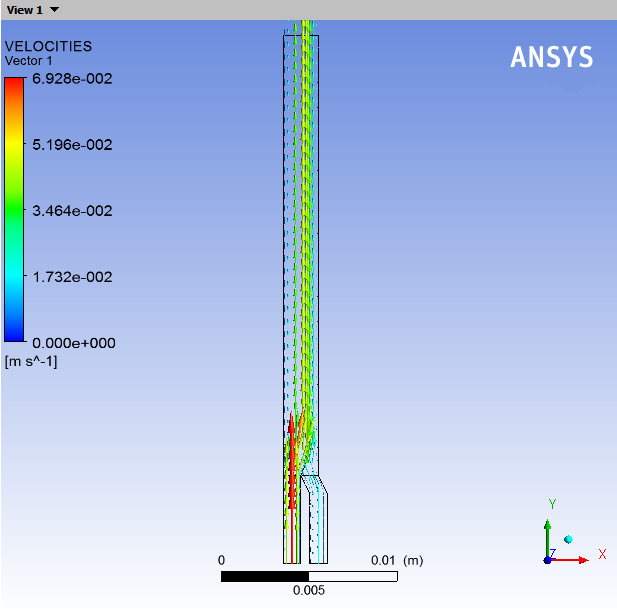
Display velocity vectors for the two fluids.
1. Deselect the contour previously defined.
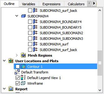
  In the Outline tree tab, under User Locations and Plots deselect Contour 1.
2. Click the Insert menu and select Vector or click the button.
3. Click OK to accept the default name (Vector 1) and display the details view below the Outline tab.
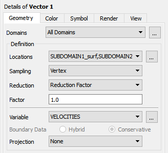
4. Perform the following steps in the details view:
  1. In the Geometry tab, click the button next to Locations.
  2. In the Location Selector dialog box that opens, select SUBDOMAIN1_surf, SUBDOMAIN2_surf, SUBDOMAIN3_surf, and SUBDOMAIN4_surf (use Ctrl for multiple selection) and click OK.
  3. Ensure that VELOCITIES is selected as the Variable.
  4. In the Symbol tab, set Symbol to Arrow3D and increase the Symbol Size to 3.
  5. Click Apply.
Figure 7.4: Velocity Vectors

Figure 7.5: Magnified View of Velocity Vectors

You can see that the velocity is continuous across the interface. As both the fluids are Newtonian, the velocity profile is a parabola on both sides of the interface. Since the force must be continuous across the interface, the shear stress generated within fluid 1 is equal to the shear stress generated within fluid 2 along the interface.

7.5. Summary

This tutorial introduced the concept of fluid layers flowing in the same duct. In Polydata, you learned how to set up a multiple-domain calculation, including the definition of a moving interface and associated remeshing methods.

The location of the interface depends largely on the physical properties of the fluids involved, the geometry of the channels, and the operating conditions (for example: flow rates of the fluids). A CFD simulation with Polyflow Classic allows you to test different setups (for example: in order to optimize the feeding of a coextrusion die).