Chapter 8: Flow of Two Immiscible Fluids by Species Method

This tutorial is divided into the following sections:

8.1. Introduction

This tutorial examines the flow of two fluids in a single die. Two polymer melts with distinct physical properties are fed through different channels into a die. The aim of the calculation is to predict the location of the interface between the two fluids.

In this tutorial you will learn how to:

Define a species.
Define a species transport problem.
Create multiple sub-tasks.
Define a PMAT function.
Define an EVOLUTION task.

8.2. Prerequisites

This tutorial assumes that you are familiar with the menu structure in Polydata and Workbench and that you have solved or read 2.5D Axisymmetric Extrusion. Some steps in the set up procedure will not be shown explicitly.

8.3. Problem Description

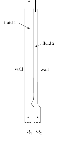
This problem analyzes the flow of two immiscible Newtonian fluids (fluid 1 and fluid 2) through a die of diameter 1 cm, as shown in Figure 8.1: A Schematic Diagram of the Two Fluids in the Die. The melts are fed into the die through boundaries 1 and 3 (see Figure 8.2: Boundary Sets and Subdomains for the Problem). The flow rates for the two fluids are not equal. The fluids come into contact in the die, creating an interface. The location of the interface is unknown and will be determined by Polyflow Classic. The location of the interface depends on the physical properties of the fluids, the flow rates of the fluids, and the geometry of the die.

Incompressibility and momentum equations are solved in the fluid domains. To determine the interface, an extra scalar transport equation is solved and material properties are made functions of this scalar using PMAT. If the scalar value is greater than 0.5, material properties of first fluid are used and if the scalar value is less than 0.5, material properties of second species are used. A Scalar value of 0.5 determines the location of interface.

Note that the same problem has been solved using the interface tracking method (see Flow of Two Immiscible Fluids).

The advantage of this method over the interface tracking method is that it can be used for more complex geometries, and it is less computationally expensive than the interface tracking method (no remeshing method must be defined). However this comes at a loss of accuracy. The interface tracking method gives a very accurate position of interface, whereas the species method produces a blurred interface.

The geometry and mesh from Flow of Two Immiscible Fluids is used.

Fluid 1 has a viscosity of = 10000 poise, and fluid 2 has a viscosity of = 5000 poise.

Figure 8.1: A Schematic Diagram of the Two Fluids in the Die

The boundary sets for the problem are shown in Figure 8.2: Boundary Sets and Subdomains for the Problem.

Figure 8.2: Boundary Sets and Subdomains for the Problem

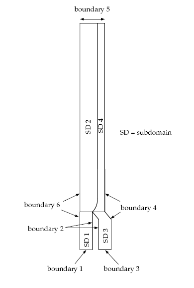
The conditions at the boundaries of the domains are:

boundary 1: flow inlet for fluid 1, volumetric flow rate = 3 cm³/s
boundary 2: outer wall common to subdomain 1 and subdomain 3: zero velocity
boundary 3: flow inlet for fluid 2, volumetric flow rate, = 1 cm³/s
boundary 4: outer wall common to subdomain 3 and subdomain 4: zero velocity
boundary 5: flow exit for both fluids
boundary 6: outer wall common to subdomain 1 and subdomain 2: zero velocity

The conditions at the boundaries of the domains for species transport:

boundary 1: scalar value equal to 1
boundary 3: scalar value equal to zero
Insulated condition at all other boundaries

Note that when using this method for a sharp interface, you should ensure that the scalar doesn't diffuse much into the domain. To ensure this, an evolution is applied on scalar diffusivity starting from a large value and gradually decreasing it to a very small number.

8.4. Setup and Solution

The following sections describe the setup and solution steps for this tutorial:

8.4.1. Preparation

To prepare for running this tutorial:

Prepare a working folder for your simulation.
Download the two_fluids_species.zip file here .
Unzip the two_fluids_species.zip file you have downloaded to your working folder.
The mesh file fluids.msh can be found in the unzipped folder.
Start Workbench from Start > Ansys 2025 R1 > Workbench 2025 R1.

8.4.2. Project and Mesh

Create a Fluid Flow (Polyflow Classic) analysis system by drag and drop in Workbench.
Save the Ansys Workbench project using File → Save, entering two-fluids-species as the name of the project.
Import the mesh file (fluids.msh).
Double-click the Setup cell to start Polydata.
When Polydata starts, the Create a new task menu item is highlighted, and the geometry for the problem is displayed in the Graphics Display window.

8.4.3. Create a Task for the Model

In the following steps you will define a single task that represents the global problem. Since this tutorial deals with two fluids, each with its own physical properties, you will need to define two different sub-tasks (one for each fluid) in the following sections.

Create a task for the model.
Create a new task
Select the following options:
- F.E.M. task
- Evolution problem(s)
- 2D axisymmetric geometry
Click Accept the current setup.

8.4.4. Species and Species Transport Sub-task

In the following steps you will define a species A and set material properties as well as boundary condition along its boundaries.

Create a species A.
Define species
Create a new species.
Create a new species
A dialog box appears asking for the name of the species.
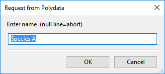
1. Enter Species A as the name of the species.
  A dialog box appears asking for the nickname of the species.
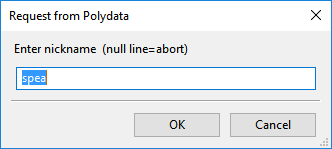
2. Enter spea as the nickname of the species.
3. Click Upper level menu.
  The Create a sub-task menu item is highlighted.
Create a sub-task for transport of the species.
Create a sub-task
1. Click Transport of species.
  Polydata asks you to select a species.
2. Click SpeciesA.
  The Domain of the sub-task menu item is highlighted.
Define the domain where the sub-task applies.
Species transport equation is solved in all the subdomains.
Domain of the sub-task
Click Upper level menu to select all of the subdomains.
Specify the material properties for species.
Material data
Polydata indicates the material properties that are relevant for the sub-task by graying out the irrelevant properties. For this model, you will only define the diffusivity of the species. The evolution will be applied on diffusivity with an initial high value (1) and decreases it to a small value (1e-9).
1. Click Diffusivity.
2. Click EVOL button at the top of Polydata menu to enable evolution inputs.
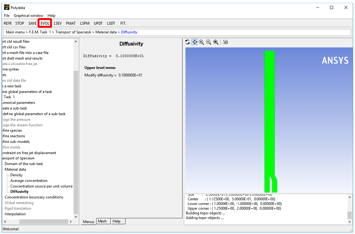
3. Click Modify diffusivity.
  A dialog box appears asking for New value of diffusivity.
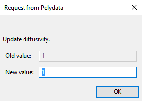
4. Click OK to accept the default value of 1.
  Polydata will take you to evolution panel. Here you will make species diffusivity a function of evolution parameter . Since the diffusivity must be decreased by several orders of magnitude, is selected.
5. Select the function f(S) = a*exp(b*S) + c + d*S.
6. Modify the value of function parameters: a, b, c, and d to 1, –20, 0 and 0, respectively.
7. Click Upper level menu.
8. Click the EVOL button at the top of the Polydata menu to disable evolution inputs.
9. Click Upper level menu twice to return to the Transport of SpeciesA menu.
  Boundary conditions of the species must be defined at all of the boundaries.
Specify the concentration boundary conditions for fluid 1 (SUBDOMAIN1 and SUBDOMAIN2).
Concentration boundary conditions
1. Set mass fraction at BOUNDARY1 equal to 1.
  1. Select Mass fraction imposed along BOUNDARY1 and click Modify.
  2. Click Mass fraction imposed.
  3. Click Constant.
    A dialog box appears asking for the new value of concentration.
  4. Set New value to 1 and click OK.
  5. Click Upper level menu.
2. Set insulated conditions at BOUNDARY2.
  1. Select Mass fraction imposed along BOUNDARY2 and click Modify.
  2. Click Insulated boundary.
3. Set mass fraction at BOUNDARY3 equal to 0.
  1. Select Mass fraction imposed along BOUNDARY3 and click Modify.
  2. Click Mass fraction imposed.
  3. Click Constant.
    A dialog box appears asking for the new value of concentration.
  4. Click OK to accept the default value of 0.
  5. Click Upper level menu.
4. Set insulated conditions at BOUNDARY4, BOUNDARY5, and BOUNDARY6.
  1. Select Mass fraction imposed along BOUNDARY4 and click Modify.
  2. Click Insulated boundary.
  3. Repeat step (i) and step (ii) for BOUNDARY5 and BOUNDARY6.
  4. Click Upper level menu twice.

8.4.5. Fluids Sub-task

In the following steps you will define the nature of the flow problem, identify the domain of definition, set the relevant material properties for fluid, and define boundary conditions along its boundaries.

Create a sub-task for the fluids.
Create a sub-task
1. Click No in the window that pops up.
  Select Generalized Newtonian isothermal flow problem.
  A dialog box appears asking for the title of the problem.
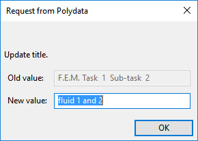
2. Enter fluid 1 and 2 as the New value and click OK.
  The Domain of the sub-task menu item is highlighted.
Define the domain where the sub-task applies.
This Sub-task is defined for all the subdomains.
Domain of the sub-task
Click Upper level menu to select all of the subdomains.
The Material data menu item is highlighted.
Specify the material data properties for fluids.
Material Data
Polydata indicates the material properties that are relevant for the sub-task by graying out the irrelevant properties. For this model, you will define only the viscosity of the material. The viscosity of material 1 will be used if the species concentration is greater than 0.5, otherwise the viscosity of material 2 will be used. This can be achieved by the use of PMAT.
1. Click Shear-rate dependence of viscosity.
2. Click Constant viscosity.
3. Click the PMAT button at the top of Polydata.
4. Specify the value for , referred to as “fac” in the graphical user interface.
  Modify fac
  Polydata prompts for the new value of .
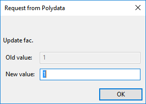
  Click OK to accept the default value of 1.
5. Polydata will take you to PMAT menu as shown below.
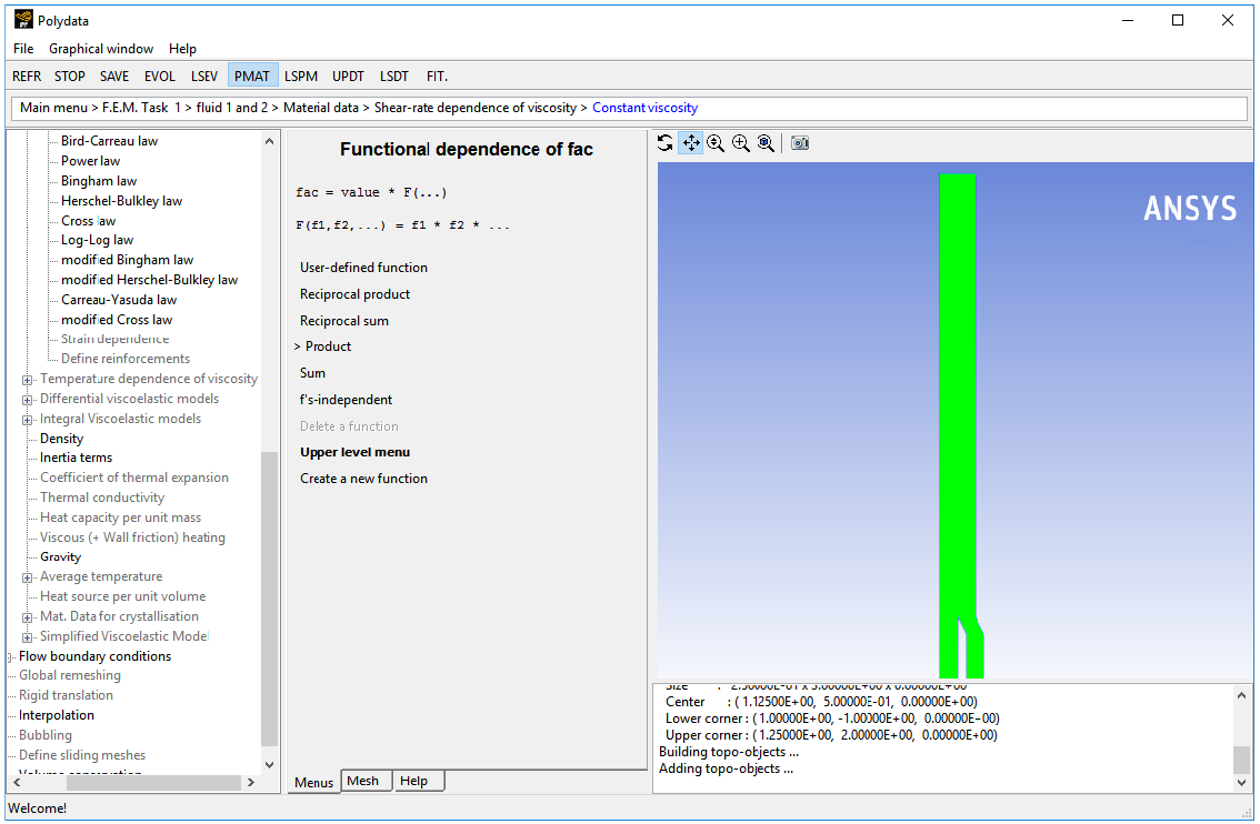
6. Create a new function.
  Create a new function
  A new function f1(...) will be created.
7. Click f1(...).
8. Select multi-ramp function.
  f(X1) = Multi-ramp function
  Polydata will ask to define pairs of values. A minimum of two pairs must be defined. Here you will define (0.495, 5000) and (0.505, 10000), where the first index stands for species concentration and the second index stands for viscosity [units: poise] value.
9. Define new pairs.
  Define new pairs (X1, f(X1))
  Polydata prompts for X1 and f(X1) sequentially.
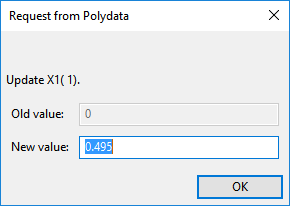
  Enter 0.495 for X1( 1), and 5000 for f(X1)( 1).
10. Define the second pair.
  Insert new pair
11. Enter 0.505 for X1( 2) and 10000 for f(X1)( 2).
12. Click Upper level menu two times.
13. Change the field to species concentration.
  Change field X1 = S (evol. var.)
14. Select SpeciesA.
15. Disable the PMAT button at the top of Polydata.
16. Click Upper level menu six times to return to the fluid 1 and 2 menu.
  The Flow boundary conditions menu item is highlighted.
Specify the flow boundary conditions for the fluids.
Flow boundary conditions
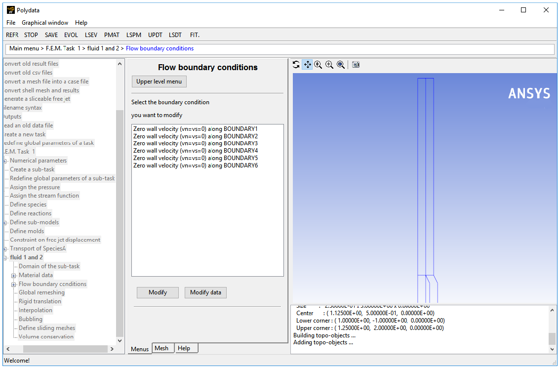
1. Set the conditions at the flow inlet for fluid 1 (BOUNDARY1).
  1. Select Zero wall velocity (vn=vs=0) along BOUNDARY1 and click Modify.
  2. Click Inflow.
  3. Click Modify volumetric flow rate.
    Polydata prompts for the new value of the volumetric flow rate.
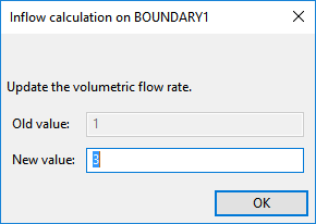
  4. Enter 3 [units: cm³/s] as the New value and click OK.
  5. Ensure Automatic is selected and click Upper level menu.
    When the Automatic option is selected, Polydata automatically chooses the most appropriate method to compute the inflow condition.
2. Retain the default condition Zero wall velocity (vn=vs=0) along BOUNDARY2.
  At a solid-liquid interface, the velocity of the liquid is that of the solid surface. Hence the fluid is assumed to stick to the wall. This is known as the no-slip assumption because the liquid is assumed to adhere to the wall, and so has no velocity relative to the wall.
  By default, Polydata imposes Zero wall velocity ( = = 0) along all boundaries.
3. Set the conditions at the flow inlet for fluid 2 (BOUNDARY3).
  1. Select Zero wall velocity (vn=vs=0) along BOUNDARY3 and click Modify.
  2. Click Inflow.
  3. Click Modify volumetric flow rate.
    Polydata prompts for the new value of the volumetric flow rate.
  4. Click OK to accept the default value of 1 [units: cm³/s] for New Value.
  5. Ensure Automatic is selected and click Upper level menu.
4. Retain the default condition Zero wall velocity (vn=vs=0) along BOUNDARY4.
5. Set the conditions at the flow outlet (BOUNDARY5).
  It is assumed that a fully developed velocity profile is reached at the exit, so the outflow condition is appropriate. This condition essentially imposes a zero normal force () that includes a pressure term, and a zero tangential velocity ().
  1. Select Zero wall velocity (vn=vs=0) along BOUNDARY5 and click Modify.
  2. Click Outflow.
6. Retain the default condition Zero wall velocity (vn=vs=0) along BOUNDARY6.
  The fluid is assumed to stick to the wall, since at a solid-liquid interface the velocity of the liquid is that of the solid surface.
7. Click Upper level menu three times to return to the top-level Polydata menu.

8.4.6. Save and Exit Polydata

Save and exit

Polydata asks you to confirm the current system units and fields that are to be saved to the results file for postprocessing.

Specify the system of units for the simulation.
1. Click Modify system of Units.
2. Click Set to metric_cm/g/s/A+Celsius.
3. Click Upper level menu twice.
Click Accept.
This confirms that the default Current field(s) are correct.
Click Continue.
This accepts the default names for graphical output files (cfx.res) that are to be saved for postprocessing, and the Polyflow Classic format results file (res).

8.4.7. Solution

Run Polyflow Classic to calculate a solution for the model you just defined using Polydata.

Run Polyflow Classic by right-clicking the Solution cell of the simulation and selecting Update.
This executes Polyflow Classic using the data file as standard input, and writes information about the problem description, calculations, and convergence to a listing file (polyflow.lst).
Check for convergence in the listing file.
1. Right-click the Solution cell and click Listing Viewer....
  Workbench opens theView listing file dialog box, which displays the listing file.
2. It is a common practice to confirm that the solution proceeded as expected by looking for the following printed at the bottom of the listing file:
```
The computation succeeded.
```

8.4.8. Postprocessing

Use CFD-Post to view the results of the Polyflow Classic simulation.

Double-click the Results tab in the Workbench analysis and read the results files saved by Polyflow Classic.
CFD-Post reads the solution fields that were saved to the results file.
Align the view.
In the graphical window, right-click, and select View from +Z under Predefined Camera.
Display contours of velocity magnitude.
1. Click the Insert menu and select Contour or click the Contour button ( ).
2. Click OK to accept the default name (Contour 1) and display the details view below the Outline tab.
3. Perform the following steps in the details view of Contour 1:
  1. In the Geometry tab, click the button next to Locations.
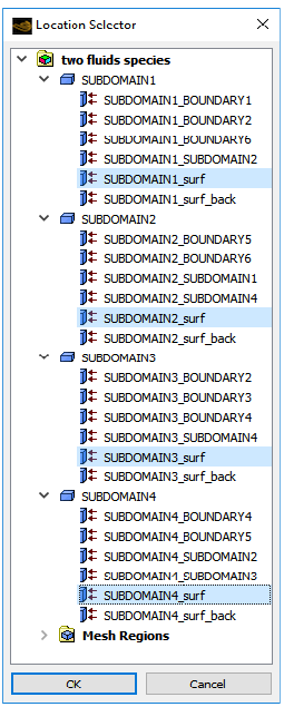
  2. In the Location Selector dialog box that opens, select SUBDOMAIN1_surf, SUBDOMAIN2_surf, SUBDOMAIN3_surf, and SUBDOMAIN4_surf (use Ctrl for multiple selection) and click OK.
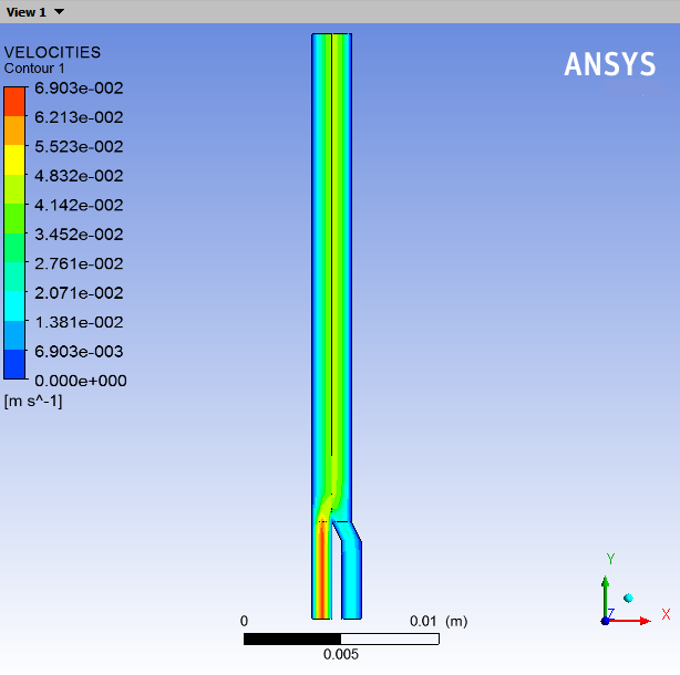
  3. Select VELOCITIES from the Variable drop-down list.
  4. Click Apply.
Figure 8.3: Contours of Velocity Magnitude

The velocity is much larger at the inlet of fluid 1 than at the inlet of fluid 2. There are two reasons for this:
- The flow rate is three times larger for fluid 1 than for fluid 2.
- You are modeling an annular die. Hence the flow section is smaller for the interior channel than for the exterior channel.
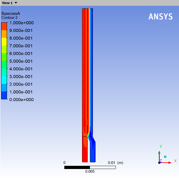
When the two fluids come into contact with each other, the interface between the two fluids is pushed towards the exterior of the annular die.
There are three reasons for this:
- The flow rate for fluid 1 is higher than for fluid 2.
- The die is annular, so even identical flow rates cause the interface to move in order to equilibrate the flow sections.
- The viscosity of fluid 1 is higher than the viscosity of fluid 2. In the process of giving more room to the most viscous fluid, its shearing decreases. This leads to a smaller global dissipation.
Display the velocity vectors for the two fluids.
1. In Outline tree tab, under User Locations and Plots, deselect Contour 1.
2. Click the Insert menu and select Vector or click the button.
3. Click OK to accept the default name (Vector 1) and display the details view below the Outline tab.
4. Perform the following steps in the details view of Vector 1:
  1. In the Geometry tab, click the button next to Location.
  2. In the Location Selector dialog box that opens, select the locations SUBDOMAIN1_surf, SUBDOMAIN2_surf, SUBDOMAIN3_surf and SUBDOMAIN4_surf (use ctrl for multiple selections) and click OK.
  3. In the Symbol tab, select Arrow 3D from the Symbol drop-down list.
  4. Set Symbol Size to 2.
  5. Click Apply.
Figure 8.4: Velocity Vectors

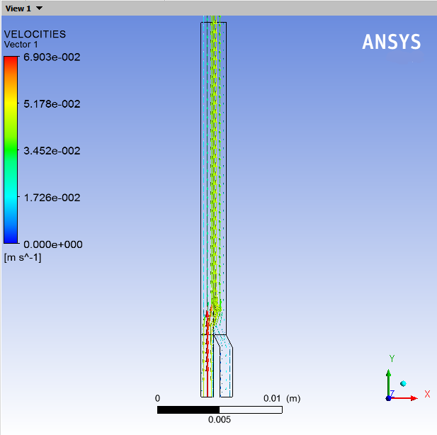
You can see that the velocity is continuous across the interface. As both the fluids are Newtonian, the velocity profile is a parabola on both sides of the interface. Since the force must be continuous across the interface, the shear stress generated within fluid 1 is equal to the shear stress generated within fluid 2 along the interface.
Displaying the contours of Species A.
1. In Outline tree tab, under User Locations and Plots, deselect Vector 1.
2. Click the Insert menu and select Contour or click the Contour button ( ).
3. Click OK to accept the default name (Contour 2) and display the details view below the Outline tab.
4. Perform the following steps in the details view of Contour 2:
  1. Click the button next to Locations.
  2. In the Location Selector dialog box that opens, select SUBDOMAIN1_surf, SUBDOMAIN2_surf, SUBDOMAIN3_surf, and SUBDOMAIN4_surf (use Ctrl for multiple selection), and then click OK.
  3. Click the button next to Variable.
  4. In the Variable Selector dialog box that opens, select SpeciesA, and then click OK.
  5. Set Range to User Specified.
  6. Enter 0 for Min and 1 for Max.
  7. Click Apply.
Figure 8.5: Contours of Species A
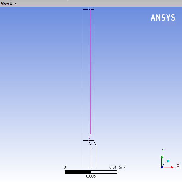
Display the interface line.
1. In Outline tree tab, under User Locations and Plots, deselect Contour 2.
2. Select Isosurface from the Location drop-down menu ( ).
3. Click OK to accept the default name (Isosurface 1) and display the details view below the Outline tab.
4. Perform the following steps in the details view of Isosurface 1:
  1. In the Geometry tab, click the button next to Variable and select SpeciesA.
  2. Enter 0.5 for Value in order to locate the interface line.
  3. In the Color tab, select Constant from the Mode drop-down list and select pink by clicking next to Color.
  4. In the Render tab, select Draw As Lines from the Draw Mode drop-down list.
  5. Click Apply.
  6. Right-click in the Graphics Window and deselect Default Legend.
Figure 8.6: Location of Interface

8.5. Summary

This tutorial introduced the concept of fluid layers flowing in the same duct. In Polydata, you learned how to set up a species transport equation, a PMAT function, and you learned how to define a coextrusion problem using species transport and PMAT functions. This method avoids the use of the remeshing method, which is computationally expensive.

The species method, although less accurate, can help in quickly finding a solution when the die has a complex shape. For more accurate results, the interface tracking method, as demonstrated in Flow of Two Immiscible Fluids, should be used. Generating a mesh for a complex die may be an issue with the interface tracking method.

The location of the interface depends largely on the physical properties of the fluids involved, the geometry of the channels, and the operating conditions (for example: flow rates of the fluids). A CFD simulation with Polyflow Classic allows you to test different setups (for example: in order to optimize the feeding of a coextrusion die).