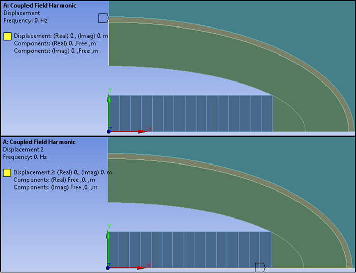
Because a quarter of the model is analyzed, two symmetry boundary conditions are applied along the x and y axes as shown below:

Figure 33.10: Symmetry Boundary Conditions

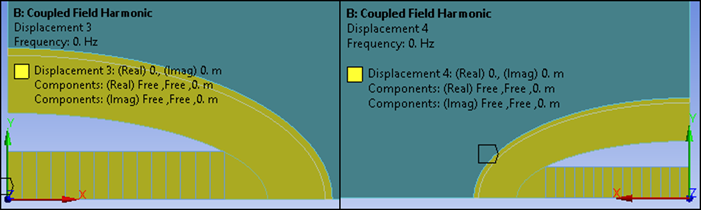
The 3D model has an additional z constraint on both planes at z = 0 and 0.01 m as shown below:

Figure 33.11: Z Constraints for 3D Model

Rigid walls and symmetry planes are naturally occurring boundary conditions in an acoustic analysis. Therefore, no acoustic boundary conditions are necessary on the two symmetry planes at x = 0 and y = 0. In the 3D case, the planar surfaces at z = 0 and 0.01 m are rigid walls and do not require boundary conditions.

2D Acoustic Wave-Absorption Condition

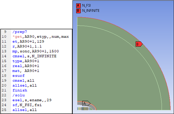
For the 2D case, the FLUID129 infinite acoustic element is used to model the wave-absorption condition. Typically, the fluid domain can be truncated around a quarter of the wavelength away from the object of interest. However, because Workbench does not support far-field postprocessing for 2D FLUID29 elements, the calculated results at 1 m must be included in the computational domain. FLUID129 elements are therefore positioned in a circular arc 1.1 m from the center.

To activate the vibroacoustic coupling, the FSI flag (SF,,FSI) is applied to the N_FSI named selection.

A command snippet is used to define the FLUID129 elements and the FSI boundary condition:

Figure 33.12: Acoustic Boundary Conditions for 2D Model

3D Acoustic Wave-Absorption Condition

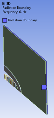
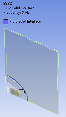
For the 3D case, the modeled domain is Cartesian. A Robin Radiation Boundary is applied to the outermost (+x and +y) surfaces to model the wave-absorption condition. Because far-field postprocessing is supported in 3D, it is not necessary for the computational domain to extend 1 m in distance. The Fluid-Solid Interface is scoped to the structural and acoustic physics interfaces.

Figure 33.13: Acoustic Boundary Conditions for 3D Model

Radiation Boundary Condition	Fluid-Solid Interface

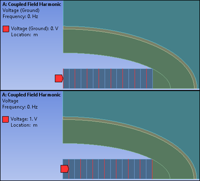
Between each piezoelectric ceramic is a terminal (not modeled). Because each terminal is equipotential, voltages of 0 V and 1 V are applied in an alternating fashion between each piezoelectric ceramic part as shown below:

Figure 33.14: Applied Voltages

Note: Make sure the polarization axis is set properly by using the local coordinate system for each piezoelectric ceramic part.