The results are analyzed to study the effect of wear on the contact conditions (contact pressure and contact area) and how wear evolves with time under steady-state loading.

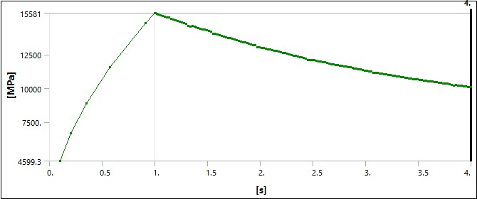
For this axisymmetric contact example, the contact condition is similar to the classical Herzian contact at the end of load step 1 (see Figure 43.11: Contact Pressure versus Time below). Wear in the hemispherical ring is activated in the second load step. The figure shows the contact pressure at the end of 300,000 rotations (3 seconds) of the hemispherical copper ring over the steel ring.

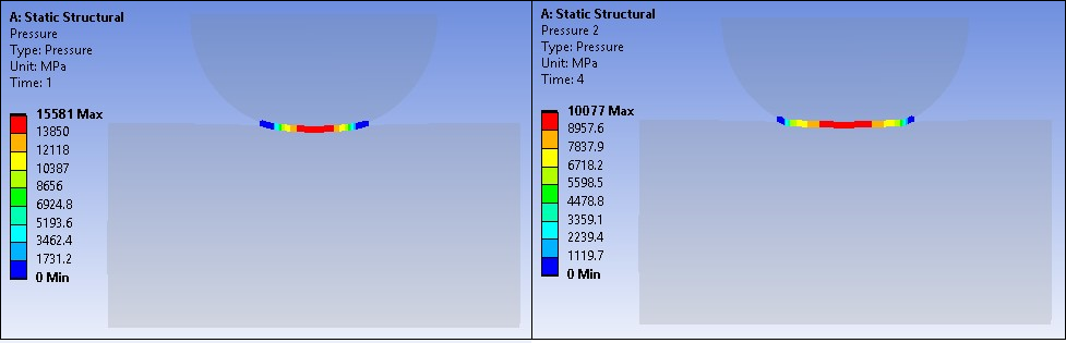
Since the amount of wear is proportional to the contact pressure, the regions with initially high contact pressure wear more and local curvature is reduced, thereby reducing the contact pressure in those regions. This also leads to an increasing area of the ring coming into contact, which increases contact pressure in regions that had low contact pressure at the beginning of the wear analysis.

Thus, the simulation captures the physical process of wear and results in an increased contact area and more uniform contact pressure. Maximum contact pressure goes down with wear and minimum contact pressure goes up with wear. That is, wear makes contact pressure more uniform as shown in Figure 43.12: Contact Pressure Before and After Wear.

Figure 43.11: Contact Pressure versus Time

Figure 43.12: Contact Pressure Before and After Wear

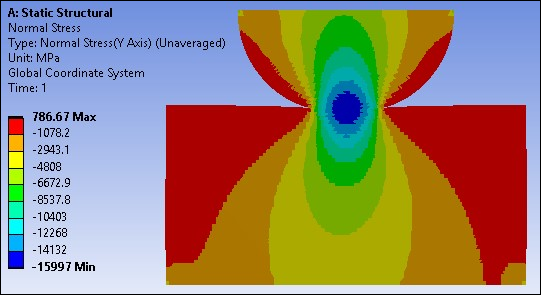
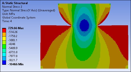
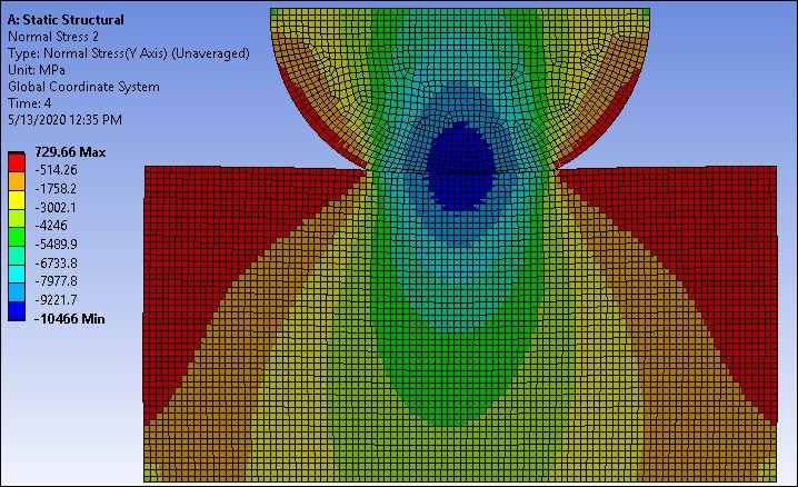
The stress in the loading (Y) direction is affected by wear in a similar way. The maximum stress decreases and the minimum stress increases, while the stress gradient is reduced. This is demonstrated in the below plots of stress before and after wear. The element distortions due to wear at the interface are also evident (see Figure 43.15: Mesh After Wear).

Figure 43.13: Normal Stress in Y Direction Before Wear

Figure 43.14: Normal Stress in Y Direction After Wear

Figure 43.15: Mesh After Wear

See Figure 43.5: 2D Axisymmetric Meshed Model to compare this mesh with the initial mesh for this model.