


Boundary conditions for the three models follow:
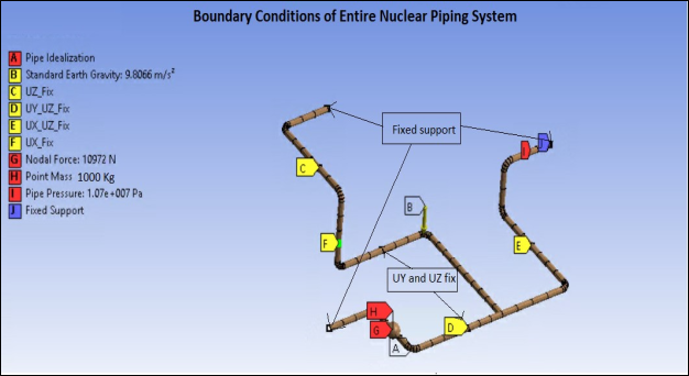
To simulate various types of supports in the system, the following boundary conditions and equivalent loading are applied:
To simulate the nozzles and anchor supports, the nodes at all three ends of the system are completely constrained.
To simulate the three two-directional supports, three nodes are constrained in either the Y and Z directions or the X an Z directions.
To simulate a horizontal support and a vertical support, two nodes are constrained respectively in the X and Z directions.
A spring hanger support is replaced by an equivalent concentrated force.
A 1000 kg mass representing a valve is simulated by a MASS21 element.
Internal pressure and gravity load are applied in the model.
8.5.2. Local Elbow Model Meshed with ELBOW290 Elements
One end of this model is fixed in all degree of freedoms and time varying displacements, representing the seismic loading condition, are applied at the other end of the elbow model, as shown in Figure 8.4: Elbow Model Meshed with ELBOW290 Elements. Internal pressure and gravity loads are identical to those applied in the global model.
8.5.3. Local Elbow Model Meshed with SHELL281 Elements
Boundary conditions for this model are identical to those applied on the local elbow model meshed with ELBOW290 elements. In this model, however, the method for applying displacement-time-history data is different.
Pilot nodes are created on both ends of the model at the center of the cross-sections. The pilot nodes are coupled with the edge nodes of the cross-sections via contact pairs. One pilot node is fixed in all degrees of freedoms and time-varying-displacement data are applied at the other pilot node, as shown in Figure 8.6: Elbow Model Meshed with SHELL281 Elements.