Go to a section topic:
Overview
The Composite Sampling Point Tool is a post-processing option that you can use for composite ply structures that were modeled using Ansys Composite PrepPost (ACP). See the Sampling Points section in the Ansys Composite PrepPost User's Guide for more information.
This tool works in tandem with the Composite Failure Tool. That is, to generate and display result data, you must scope the Composite Sampling Point Tool to existing Composite Failure Criteria. This criteria is created by promoting a defined Composite Failure Tool object. Be sure to review the Composite Failure Tool section as it is a prerequisite for using this feature.
Also see the Composite Sampling Point object reference section.
Application
To define results using the Composite Sampling Point Tool:
Make sure that your composite analysis is properly defined.
Define and promote a Composite Failure Tool.
With the Composite Failure Tool selected, right-click and select > > . The application inserts a Composite Sampling Point Tool object. It is automatically the active object and by default, includes the child object Composite Sampling Point.
Note: You can also insert a by right-clicking the Solution object or in the geometry windows and selecting > > .
Specify the property. The Worksheet displays automatically and contains the criteria as specified in the object.
Select the Composite Sampling Point child object.
Using the Geometry property, select the desired faces on your geometry. The sampling point is created at the location of hit point on the geometry face and the direction of the sampling point is aligned with the face normal.
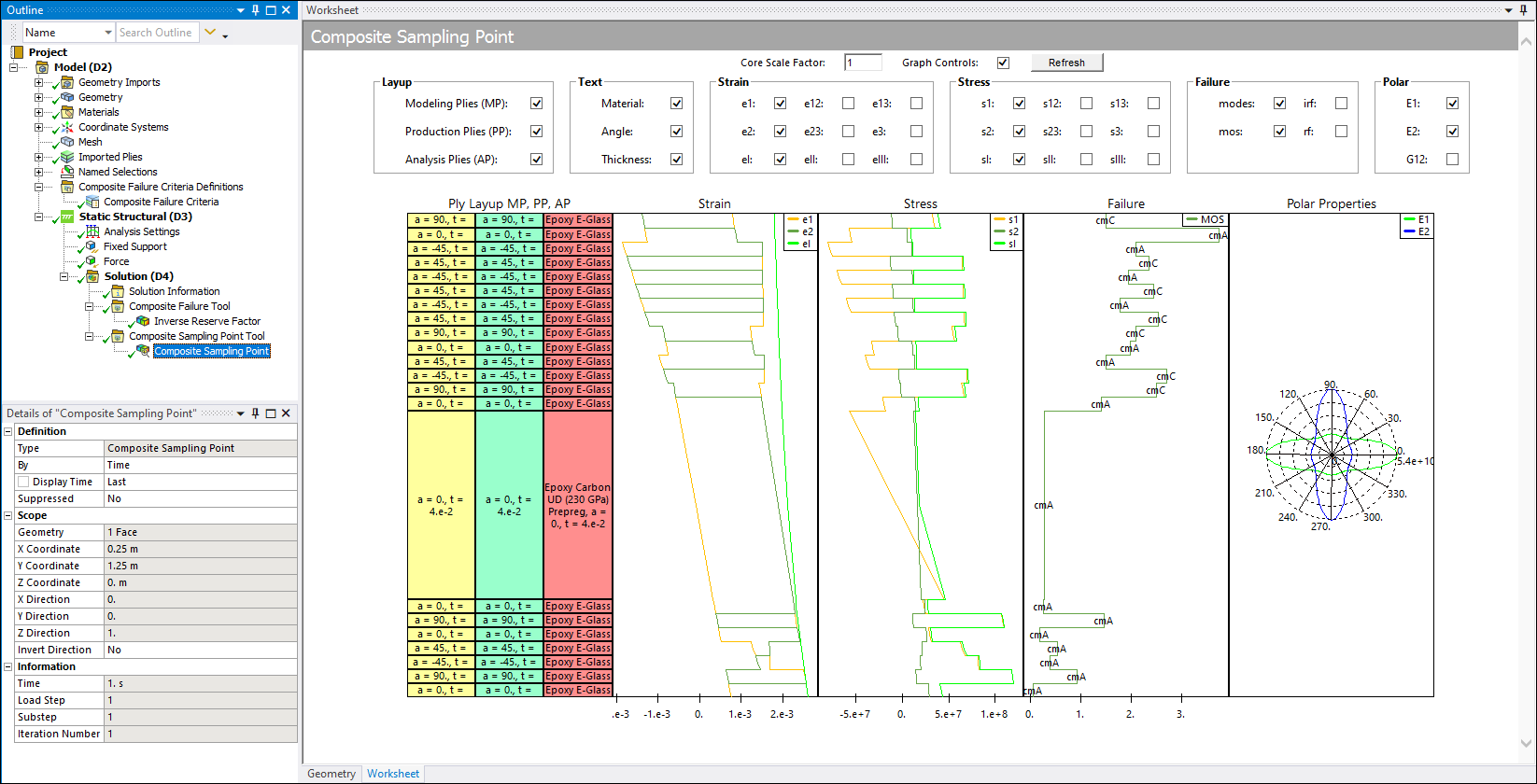
Solve or evaluate the results of the analysis. Once complete, the Worksheet displays automatically. Select desired result data from the available options (Layup, Text, Strain,, etc.). The example worksheet show below illustrates result data. This example illustrates that you can use the Text group to display the material, thickness, and angle as text labels for every ply in the plot. The angle displayed for modeling and production plies always matches the design angle in the modeling ply and material definitions.
Note: The worksheet does not display result content using the units specified in the Units option.
Worksheet Display
The Worksheet displays the thickness distributions using the options of the Layup group as well as the post-processing results (Strain, Stress, and Failure groups) as 2D plots. Stresses and strains shown in the 2D plot display the values at the interpolated element center at the top and bottom of the layer. The 2D failure plot shows the worst IRF, RF or MoS factor of all failure criteria, failure modes evaluated, and integration point level. In addition, the display can show failure modes as text labels for every ply. And you can enable the polar properties of the laminate using the options of the Polar Properties group. In addition, there are several worksheet user interactions available, including:
Left Mouse Button: Select and hold to move the content of all columns vertically. Select and hold on an individual column to move content horizontally.
Mouse Wheel: This key zooms in and out on the vertical axis of all columns. Combine this action with the [ctrl] key to zoom in and out along the horizontal axis on individual columns.
Right Mouse Button: Place the cursor over a graph location and then right-click and hold to display a tooltip that includes comma separated values for a stress, strain, failure, (left tooltip value) and a thickness (right tooltip value) for that associated worksheet value.
Core Scale Factor: This entry visually scales the core layer's thickness in order to allow more space within the columns to draw the other layers. This is especially useful when the core layer is much larger than other layers. The default value is 1. You can enter smaller values incrementally to reduce the size of the displayed core layer.
Escape Key: Reset all charts to original view.
Note: The Polar Properties chart does not support user interactions.