


This section discusses the options available when selecting degrees of freedom (DOFs) in a rigid body assembly and their effect on simulation time.
The double pendulum model shown below is considered in this section. The first body in this model (in blue) has center of gravity G1. This body is linked to the ground through revolute joint R1, and linked to a second body through revolute joint R2. The second body (in red) has center of gravity G2, and is linked to the first body through revolute joint R2.
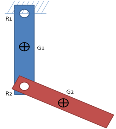
The two bodies in this model are rigid, meaning that the deformations of these bodies are neglected. The distance between any two points on a single rigid body is constant regardless of the forces applied to it. All the points on the body can move together, and the body can translate and rotate in every direction.
Many parameters are available to describe the body position and orientation, but the parameter usually chosen for the translation is the position of the center of mass with respect to a ground coordinate system. It is extremely difficult to represent 3D rotations for the orientation in a universal way. A sequence of angles is often used to describe the orientation, but some configurations are singular. An option frequently used to describe the orientation in computer graphics is the use of quaternion (also known as Euler-Rodrigues parameters); however, this option uses four parameters instead of three, and does not have a simple interpretation.
A natural choice of parameters to describe the position and orientation of the double pendulum model, is to use the position and orientation of the two individual bodies. In other words, use three translational and rotational degrees of freedom for each body, and introduce the joints using constraint equations.
The constraint equations used state that the two points belonging to the two bodies linked by the revolute joint are always coincident, and that the rotation axis of the joint remains perpendicular to the other body. This requires five constraint equations for each revolute joint.
The selected degrees of freedom (six DOFs per body and certain joints based on constraint equations) are considered "absolute" parameters.
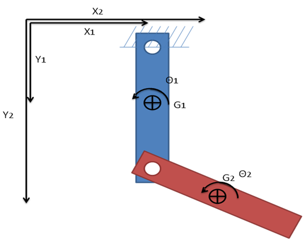
The model shown in Figure 5.4: Absolute Degrees of Freedom depicts global parameters in 2-D for the double pendulum. Body 1 and 2 are respectively parameterized by X and Y translation and theta rotation. Because the model has only two degrees of freedom, it does not require any additional constraint equations.
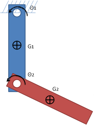
Global parameters for the body are chosen independently of the joints that exist between those bodies. When these joints are known, parameters for the joints can be chosen that reduce the number of parameters and constraint equations needed. For this example, the first degree of freedom is defined as the relative orientation of the first body with respect to the ground. The second degree of freedom is defined as the relative orientation of the second body with respect to the first body. Relative degrees of freedom are shown in the figure below:
Next, a third body is added to the model that is grounded on one side and linked to the second body with another revolute joint, as shown below:
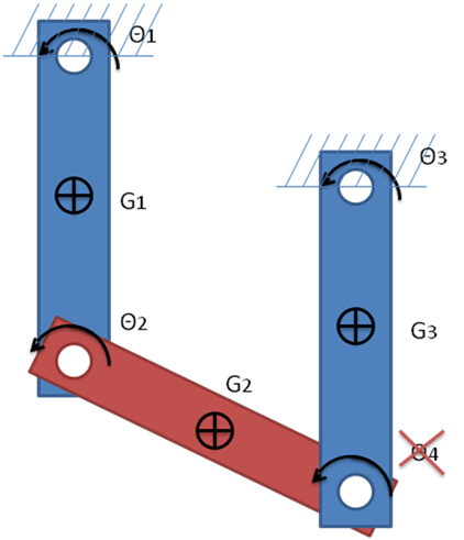
The closed loop model shown above has three bodies (plus the ground) and four revolute joints. The degrees of freedom can be chosen for the example as follows:
| Θ1 - The relative rotation of body 1 with respect to ground |
| Θ2 - The relative rotation of body 2 with respect to body 1 |
| Θ3 - The relative rotation of body 3 with respect to ground |
The fourth revolute joint cannot be based on degrees of freedom because both the motions of Body 2 and Body 3 are already defined by existing degrees of freedom. For this joint, constraint equations are added to the relative degree of freedom parameters.
Θ1, Θ2, and Θ3 will be the degrees of freedom, and the corresponding joints will be topological joints. The fourth joint will be based on a constraint equation. Constraint equation-based joints are also known as kinematic joints. Kinematic joints are needed when the model has closed loops, that is, when there is more than one way to reach the ground from a given body in the system.
To determine which joints will be topological joints and which will be kinematic joints, a graph is constructed to show connections where the bodies are vertices and the joints are arcs. This graph is decomposed into a tree, and the joints corresponding to arcs that are not used in the tree are transformed into kinematic joints.
The Model Topology view displays whether joints are based on degrees of freedom or constraint equations.
Kinematic Variables vs. Geometry Variables
Euler's theorem on rotations states that an arbitrary rotation can be parameterized using three independent parameters. The choice of these three parameters is not unique, and many choices are possible. For example:
A sequence of three rotations, as introduced by Euler (the first rotation around X, the second rotation around the rotated Y' axis, and the third rotation around the updated Z'' axis). Many other sequences of rotations exist, among them the Bryant angles.
The 3 components of the rotation vector
Etc…
Unfortunately, these minimal sets of parameters are not perfect. Sequences of angles usually have some singular configurations, and the composition of rotations using these angles is simple. This composition of rotation is intensively used in transient simulation. For example, it can be used to prevent the use of the rotation vector.
Another option is to use the 3x3 rotation matrix. Composition of rotations is easy with this option, as it corresponds to matrix multiplication; however, this matrix is an orthogonal matrix, and time integration must be done carefully to maintain the matrix properties.
A good compromise is to use quaternion, which have 4 parameters and a normalization equation.
Once rotation parameters have been selected, the time derivatives of these parameters have to be established:
 | (5–7) |
where  is the angular velocity vector.
Two sets of variables exist:
Kinematic variables, expressed as {q}:
 as long as the translational velocities.
Geometric variables, expressed as {g}, as well as the position variables for the translations. The geometric variables are obtained by time-integration of the kinematic variables.