


So far, the only interaction between bodies that has been considered was permanent joints; however, impacts and contacts will also play a significant role.
Contact Kinematics
The figure below depicts the contact between convex bodies j and k.

The non-penetration equation below describes the contact between these bodies, and is written along the shared normal at the contact point:
 | (5–82) |
In this equation, the two points Mj and Mk are the points that minimize the distance between the two bodies, and thus are not material points, that is, their location varies over the bodies with time.
For more information on the definition of the contact point, refer to Pfeiffer [PFE96] in References.
Special Cases
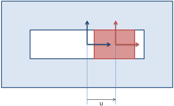
Some special cases are worth mentioning. For instance, when contact occurs in a joint between two bodies linked by that joint, the contact points become material points, and Equation 5–82 can become dependent on one single degree of freedom. Figure 5.12: Stops on a Translational Joint shows an example of stop on a translational joint. Both left and right vertical surfaces can impact the red body, but this translates very easily into a simple double inequality:
 | (5–83) |
where subscript m stands for the minimum bound, and M stands for the maximum bound. The normal here is replaced by the projection on the joint degree of freedom.
Another case of specialized contact geometry is the radial gap where contact points can be computed explicitly. In the general case of complex geometries, the strategy for computing the contact points and the impact times is more complex.
General Cases
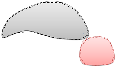
In general cases, geometries that are potentially in contact are neither simple nor convex. It is however required to find the accurate position of the contact points between two bodies. Sometimes the contact point is unique, as shown in the figure below.
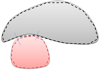
But for the same pair, the contact can occur in more than one point, as shown in the figure below.
Finally, the contact can exist along a full line for some geometries, or even on an entire surface, as shown in the figure below. In this case, there is an infinite number of contact points.

Contact Formulation
Two bodies will impact when their distance is equal to zero. Once the distance is equal to zero and the bodies are touching, forces can develop in the contact. When the contact distance is greater than zero, there is no interaction between the bodies. Introducing interaction in the equations of motion results in the addition of inequalities to the system:
 | (5–84) |
where the subscript u stands for unilateral.
In the Rigid Dynamics solver, contact and stops always use a pure Lagrange formulation. Unlike the penalty based approaches, pure Lagrange prevents any penetration.
Note: Although a pure Lagrange formulation prevents penetration, a small penetration (linear with the time step) may be visible when using the MJ Time Stepping time integration due to the lack of exact collision detection.
Rigid Contact Detection
To control the density of contact points that will need to be adjusted, a surface mesh is used on the bodies that has contact defined. Mesh based contact points are first computed.
When the contact is geometry-based, these discrete points are then adjusted on the actual geometrical surfaces.
Based on whether the contact is geometry-based or mesh-based, the requirements in terms of mesh are different:
- Geometry-Based Contact
It is important to understand that contact will create constraints between the two bodies. The relative motion between these two bodies varies in a 6-dimensional space, so 6 contact points at most will be used to constrain the relative motion of two bodies. These constraints will be added to already existing constraint, so contact can create additional redundancies. For example, two cams with parallel axis will contact along a line (as shown in the figure below). However, if the two axes are maintained parallel by existing joints in the model, one single point through the thickness of the cam is necessary to properly represent the kinematics of the assembly. To avoid useless calculation, the mesh through the thickness can be coarse.
If the mesh is very refined, many points through thickness can satisfy the contact equations. An automatic filtering of the contact points will also be performed, but the position of the points through thickness might vary from one step to the next. This can cause some unexpected changes in the moment developed in the contact. To avoid this situation, it can be useful to modify the joints or the geometry itself, and include a draft angle in the cam profile extrusion for force the contact along a line.
- Mesh-Based Contact
Similar to geometry-based contact, the mesh defines the density of contact points defined between the bodies. Because the points are on the mesh and not on the geometry, the contact happens between faceted geometries. To avoid spikes in the forces, it is recommended that you refine the mesh further when contact is mesh-based.
Caution: When the mesh-based contact detection method is used, the behavior of the contact is not symmetric. Results may change when the contact is flipped.
Using mesh-based contact with Runge-Kutta may lead to computationally expensive simulations. Mesh-based contact is recommended for use with the Moreau-Jean method.
Time Integration and Contact
In the Rigid Dynamics solver, two alternate methods are available. The first method is suited for situations where contact is mostly intermittent, the second method is suited where contact is mostly established, for example the contact involved in a pair of gears.
- Method 1: Event Capturing Contact Formulation
A second method of contact formulation is to detect the transition between the separated space of a given pair of bodies and the configuration where they are overlapping. The image below depicts a point mass approaching a separate wall, and the overlapping configuration following impact.
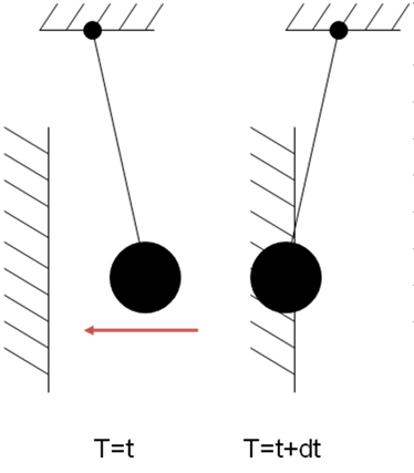
Determining the time of the transition using this point mass model involves advancing in time without introducing non-penetration constraint equations, and realizing at the end of the time step that the penetration is not acceptable. By using the polynomial interpolation that the time integration scheme provides over the time step, the moment where the penetration reaches zero can be found fairly accurately. This time value can be expressed as a fraction of the time step. To determine this time value, find α such that p(t+αΔt)=0 where p is the penetration distance.
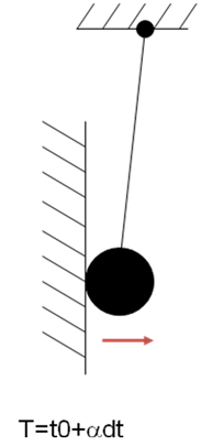
Advancing in time up to αΔt will position the system exactly at the impact time and position, where an impact occurs between the bodies. This impact is assumed to have a very short duration, orders of magnitude smaller than the simulation time. During the impact, the interaction forces between the bodies are first increasing in a compression phase, and then decreasing in the expansion phase until they vanish entirely. This impact will lead to a certain amount of energy loss determined by the material of the bodies interacting.
Newton’s impact laws are idealized in this impact process. They relate the relative velocity before the impact to the "bouncing" velocity after the impact using a restitution factor. This restitution factor varies from zero to one. A restitution factor of one indicates that the normal velocity after the impact is equal to the velocity before the impact.

(5–85)
Where the superscript + represents quantities after the impact, and the superscript – represents quantities before the impact.
A restitution of zero leads to:

(5–86)
And the general formula will be:

(5–87)
where r is the restitution factor.
This equation is written as a scalar equation at the impact point. Combined with the conservation of momentum it leads to the following system:
M(g,t){Δq}={0}
B(q){Δq}=0 for all permanent equations and active contacts, and B(q){Δq}=–(1+r)v– for the impacting contact.
Each impact with a restitution factor less than one will introduce an energy loss in the system. In a model with multiple imperfect impacts over time, the total energy will be constant piecewise with a drop at each impact.
Runge-Kutta 4, Generalized-α, and Stabilized Generalized-α integration methods are event capturing schemes (see the table below).
- Method 2: Event Absorbing Contact Formulation
When the density of events increases (small bounces, with phases where the contact is sliding, such as the contact in a pair of gears) the event detection method starts to lose efficiency and robustness, for two reasons:
It requires accurate detection of the transition time, thus forcing the reduction of the time step to avoid missing changes. If events are changed, inconsistencies between the state of the contact (whether the contact is touching, separated, or in-between) and the actual relative position of the bodies.
Each event processing phase has a computational cost.
To work around these difficulties, it is possible to reformulate what happens during the time step in terms of variation of velocities. These variations come from both smooth dynamics (the variation due to finite accelerations) and from non-smooth dynamics (the variation due to infinite accelerations over a zero duration, which corresponds to a shock). For specific theory information, see Moreau-Jean Method.
MJ Time Stepping is an event absorbing scheme.
- Summary of Time Integration Methods
The following table summarizes the characteristics of the Time Integration Types available for the Rigid Dynamics solver and the corresponding recommended setting for the Contact Detection.
Time Integration type RK4, Generalized-α, Stabilized Generalized-α MJ Time Stepping Event treatment Event capturing Event absorbing RBD Contact Detection Geometry based Best choice Not recommended Mesh based Not recommended Best choice Note: When the Time Integration Type is set to Program Controlled, the Rigid Dynamics solver chooses the time integration type based only on the use of flexible parts, regardless of the contact definition. If the contact uses only rigid bodies, the solver will use RK4. If there are any Condensed Parts, it will use Stabilized Generalized-α. The contact definition has no influence on this logic.
The use of mesh-based contact detection with explicit time integration (RK4) is likely to lead to solver problems and is not recommended.
When two Parts come into contact with zero relative velocity but non-zero absolute velocity or a load is applied to one of them, unwanted penetration may occur. This can be circumvented by reducing the time step.