Once you insert a Fatigue Tool object into your analysis, you select from the result options listed below. By default, the results are scoped to . However, you can modify scoping and apply it to individual parts or faces as desired. If you are working with a shell model, note that the application always specifies the top face value.
The result options are provided on the Fatigue Tool Context menu or by right-clicking on the object and selecting > [desired result].
Note: The application does not support the Fatigue Tool when you have symmetry specified in the analysis.
| Contour Results | Graph Results |
|---|---|
Life
This result contour plot shows the available life for the given fatigue analysis. If loading is of constant amplitude, this represents the number of cycles until the part will fail due to fatigue. If loading is non-constant, this represents the number of loading blocks until failure. Thus if the given load history represents one month of loading and the life was found to be 120, the expected model life would be 120 months.
During a constant amplitude analysis, if the alternating stress is lower than the lowest alternating stress defined in the S-N curve table, the application uses the Life result for that point. In addition, for this case, the application imposes a limit of 1e06 cycles if the Linear S-N curve definition is used.
Damage
Fatigue damage is defined as the design life divided by the available life. The default design life may be set through the Options dialog box. A damage of greater than 1 indicates the part will fail from fatigue before the design life is reached.
Note: When you set the Type property to , and specify a result, the damage per stress cycle is the reciprocal value of the Infinite Life property value if the stress cycle is below the Endurance limit. As a result, loading histories that have numerous stress cycles below the endurance limit may exhibit a greater accumulated damage value than expected. You can mitigate this effect by setting a high Infinite Life value.
Safety Factor
This result is a contour plot of the factor of safety (FS) with respect to a fatigue failure at a given design life. The maximum FS reported is 15.
These are the steps at each node to calculate Safety Factor:
Calculate the alternating and mean stress tensor.
Collapse alternating and mean stress from tensor to scalar using selected stress component.
Calculate Safety Factor from the mean stress equation using Seqv as queried from the SN curve for the design life.
1/FS = Salt/Seqv + SMean/SUltimate
Biaxiality Indication
This result is a stress biaxiality contour plot over the model that gives a qualitative measure of the stress state throughout the body. Note the following biaxiality values:
-1= Pure shear0= Uniaxial stress1= Pure biaxial state
For non-proportional loading, specify the desired biaxiality using the Method property. Options include:
: The application will sum the biaxiality for both single load cases and divide by 2.
: This calculation is the difference between single load case biaxiality and Average biaxiality. Therefore, a small Standard Deviation indicates behavior that is close to proportional loading whereas a large Standard Deviation indicates a significant change in the principal stress directions.
Equivalent Alternating Stress
The equivalent alternating stress is the stress we use to query the SN curve after accounting for multiaxial loading and mean stress effects. This result is not valid if the loading has non-constant amplitude, (that is, Loading Type = ). The result is useful for cases where the design criterion is based on the equivalent alternating stress that you specify.
These are the steps at each node to calculate Equivalent Alternating Stress:
Calculate the alternating and mean stress tensor.
Collapse alternating and mean stress from tensor to scalar using selected stress component.
Calculate the Equivalent Alternating Stress using the desired empirical stress theory, as specified by the Mean Stress Theory property of the Fatigue Tool object. For example, when you set the Mean Stress Theory property to Goodman, the Equivalent Alternating Stress calculation becomes:
EqvAltStress = Salt/(1 - SMean/SUltimate)
Therefore, that is the value reported as Equivalent Alternating Stress and this is used to query Fatigue Life from the SN Curve.
Important: If you specify a Mean Stress Theory and static failure is predicted, the reported equivalent alternating stress is reported as 1e32 Pa (this value is always reported when there is static failure).
Rainflow Matrix (History Data only)
This graph depicts how many cycle counts each bin contains. This is reported at the point in the specified scope with the greatest damage.
The Navigational Control at the bottom right-hand corner of the graph can be used to zoom and pan the graph. You can use the double-sided arrow at any corner of the control to zoom in or out. When you place the mouse in the center of the Navigational Control, you can drag the four-sided arrow to move the chart points within the chart.
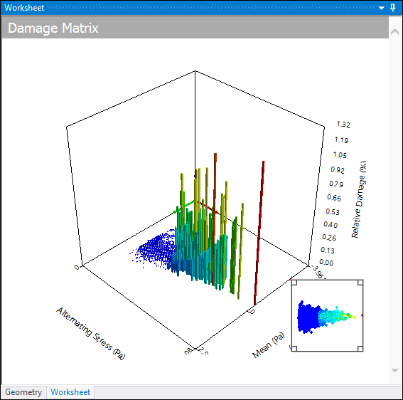
Damage Matrix (History Data only)
Similar to the rainflow matrix, this graph depicts how much relative damage each bin has caused. This result can give you information related to the accumulation of the total damage (such as if the damage occurred though many small stress reversals or several large ones).
The Navigational Control at the bottom right hand corner of the graph can be used to zoom and pan the graph. You can use the double-sided arrow at any corner of the control to zoom in or out. When you place the mouse in the center of the Navigational Control, you can drag the four-sided arrow to move the chart points within the chart.
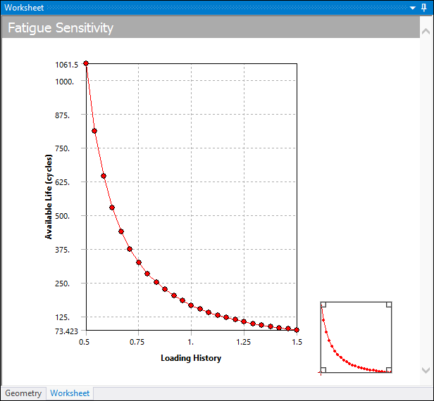
Fatigue Sensitivity
This plot shows how the fatigue results change as a function of the loading at the critical location on the scoped region. Sensitivity may be found for life, damage, or factory of safety. For instance, if you set the lower and upper fatigue sensitivity limits to 50% and 150% respectively, and your scale factor to 3, this result will plot the data points along a scale ranging from a 1.5 to a 4.5 scale factor. You can specify the number of fill points in the curve, as well as choose from several chart viewing options (such as linear or log-log).
The Navigational Control at the bottom right hand corner of the graph can be used to zoom and pan the graph. You can use the double-sided arrow at any corner of the control to zoom in or out. When you place the mouse in the center of the Navigational Control, you can drag the four-sided arrow to move the chart points within the chart.
To specify a result item, you must be under a Solution object.
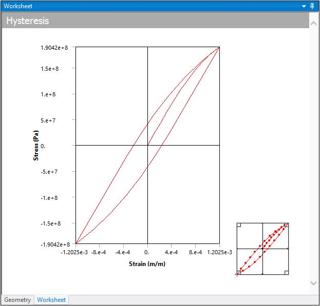
Hysteresis
In a strain-life fatigue analysis, although the finite element response may be linear, the local elastic/plastic response may not be linear. The Neuber correction is used to determine the local elastic/plastic response given a linear elastic input. Repeated loading will form close hysteresis loops as a result of this nonlinear local response. In a constant amplitude analysis a single hysteresis loop is created although numerous loops may be created via rainflow counting in a non-constant amplitude analysis. The Hysteresis result plots the local elastic-plastic response at the critical location of the scoped result (the Hysteresis result can be scoped, similar to all result items). Hysteresis is a good result to help you understand the true local response that may not be easy to infer. Notice in the example below, that although the loading/elastic result is tensile, the local response does venture into the compressive region.
Loading/Elastic Response
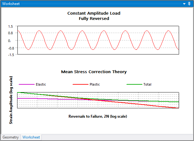
Corresponding Local Elastic Plastic Response at Critical Location