


The following topics are discussed:
- 9.2.2.1. Creating a Low Pressure Ratio Compressor Impeller
- 9.2.2.2. Initial Design Parameters - Compressor Impeller
- 9.2.2.3. Initial Angle/Thickness Parameters
- 9.2.2.4. BladeGen Layout
- 9.2.2.5. Optimizing the Meridional View
- 9.2.2.6. Define the Hub and Shroud Profiles in the Meridional View
- 9.2.2.7. Adjust the Blade Angles at the Hub in the Angle View
- 9.2.2.8. Adjust the Blade Angles at the Shroud in the Angle View
- 9.2.2.9. Define the Blade Thickness Profile
- 9.2.2.10. Prescribe the Leading/Trailing Edge Ellipse
- 9.2.2.11. Viewing the Design in the Auxiliary View
- 9.2.2.12. Saving Your Model
The following procedure can be followed as an example of using BladeGen to create a Low Pressure Ratio Compressor Impeller from start to finish.
Please note that a significant advantage of BladeGen is in the flexibility of its operations. This example will guide the user through a simple example utilizing Angle/Thickness mode and is not to be taken as the only way to use BladeGen.
BladeGen allows the user to create a blade system from scratch, using one of six standard initial configuration types. For this example, a Radial Impeller is used.
Select the File | New | BladeGen Model menu command or
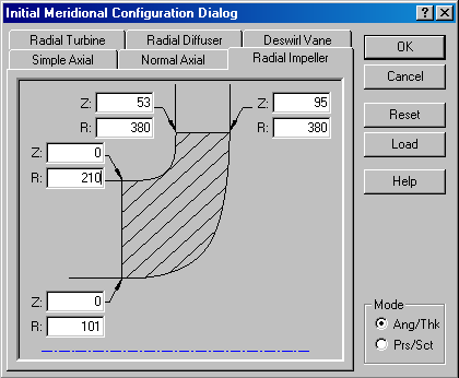
 toolbar button which will display the Initial Meridional Configuration Dialog (shown in Figure 9.74: Initial Meridional Configuration Dialog Box).
Select the Radial Impeller tab.
Enter the parameters for the initial blade layout as shown in Figure 9.74: Initial Meridional Configuration Dialog Box.
Be sure to select Ang/Thk mode in the bottom right corner
Press Enter or select the OK button to continue.
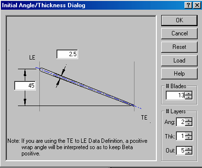
Using Figure 9.75: Initial Angle/Thickness Dialog , the initial blade parameters are completed:
Enter the nominal wrap angle of 45 degrees, thickness of 2.5 and 13 blades. Normally, BladeGen sets the leading edge theta to zero. If the Data Direction is set to TE to LE in the User Preferences Dialog, then the trailing edge theta is set to zero.
Press Enter or select the OK button to display the BladeGen Window.
The following topics are discussed:
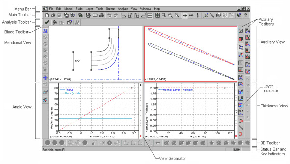
After the initial parameters have been specified, the typical BladeGen layout will be opened. The two views in the top row are the Meridional View and Auxiliary View. The bottom row has the Angle View and the Thickness View. .
In general, it is suggested that users first define the meridional profile before defining the Ang/Thk or Prs/Sct views, since these views are dependent on the path length of the meridional profile.
BladeGen uses a common set of mouse functions to manipulate the views. These functions are described in Common Mouse Functions .
The following topics are discussed:
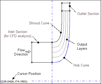
The most critical operation in the meridional view is to define the shape of the hub and shroud curve. The endpoints for these curves were specified when Initial Design Parameters (Initial Design Parameters - Compressor Impeller ) were entered. The location of a point can be easily visualized by utilizing the hover help. The bubble is displayed when the user holds the mouse cursor stationary (hovers) over a data point. When required, the location of a point can be changed in two ways:
To interactively move a point:
Click the desired point and hold the mouse button down.
Move the mouse until the point is at the intended location.
Release the mouse button
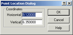
Double-click the mouse button on the intended point.
The Point Location dialog box will open as shown in Figure 9.78: Point Location Dialog Box.
Enter the intended co-ordinate values.
Click OK.
The hub and shroud profile for this case are well defined automatically. In this case, there is no need for any additional modifications.
The following topics are discussed:
The meridional profile is now defined and the Blade angles can be set. In the Angle View, the active layer is indicated by a red dot in the layer column on the right-hand side. By default, the hub layer is active. Once the Hub angles are set, the Shroud layer can be activated by left-clicking the black dot at the top of the layer column.
The blade angles can now be defined as follows:
Right-click in the Angle view and select Adjust Blade Angles.
In the Leading Edge tab, enter 47° for the Tangential Beta value, the Beta value will automatically be updated as 90° minus Tang. Beta. Leave all the other values at zero.
In the Trailing Edge tab, enter a Theta angle of 32.2° and enter 30° for the Beta value. The Tangential Beta value will be automatically updated as 60°. All other values can remain as zero.
Close the Blade Angle Dialog by selecting OK.
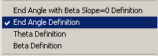
There are 4 ways to set the angle definitions. In this example, the End Angle Definition will be used. Right-click in the Angle view and select End Angle Definition as shown in Figure 9.79: Blade Angle Definition. This option applies the End-Angle definition described above, with an additional restriction that sets the slope of the Beta curve to zero at the leading and trailing edges.
The following topics are discussed:
Make the Shroud layer active by selecting the black dot at the top of the layer column. It will turn red and the Shroud is now active.
Right-click in the Angle view and select Adjust Blade Angles
In the Leading Edge tab, enter 27.5° for the Tangential Beta value. Leave all the other values at zero.
In the Trailing Edge tab, enter a Theta angle of 28.9° and 60° for the Tangential Beta. The Beta value will be automatically updated as 30°. All other values can remain as zero.
Close the Blade Angle Dialog by selecting OK
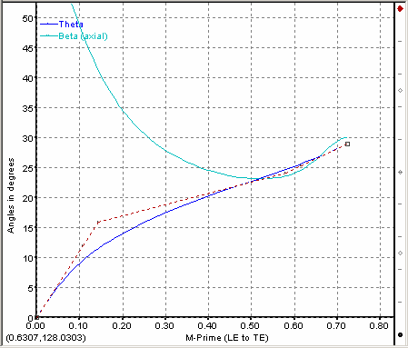
Right-click in the Angle view and select End Angle Definition as shown in Figure 9.79: Blade Angle Definition. The angle view should now look like the view shown in Figure 9.80: Shroud Angle Definition. Note that the new blade shape is automatically updated in the Auxiliary view.
At this time, the Blade thickness can be defined in the Thickness view. For this example, a constant thickness of 2.5 will be used and no modifications are required. When modifications to this curve are required, curve and point modifications can be applied.
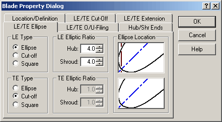
Select Blade | Properties menu commands or the ![]() toolbar button located on the left hand side of the BladeGen window to set the blade properties. Set the Leading Edge/Trailing Edge Ellipse tab; adjust the values as shown in Figure 9.81: LE/TE Ellipse Settings. All other values can remain unchanged.
toolbar button located on the left hand side of the BladeGen window to set the blade properties. Set the Leading Edge/Trailing Edge Ellipse tab; adjust the values as shown in Figure 9.81: LE/TE Ellipse Settings. All other values can remain unchanged.
Thus far, the Auxiliary view has been showing the Blade-to-Blade view. It is also helpful to display the 3D shape of the blade. To do so, use the View | Auxiliary View Content | 3D View menu command or the ![]() toolbar button located on the right side toolbar. Use the left mouse button to rotate the view, right mouse to pan and the wheel on a wheel mouse to zoom in and out.
toolbar button located on the right side toolbar. Use the left mouse button to rotate the view, right mouse to pan and the wheel on a wheel mouse to zoom in and out.
Table 9.15: 3D View Display Options
|
Menu Command |
Button |
Description |
|---|---|---|
|
Wireframe |
|
Shows the curves that define the edges of the surfaces. |
|
Meshed |
|
Shows the surface mesh from which the shaded surfaces and volume mesh will be defined. |
|
Shaded |
|
Shows opaque surfaces defined by the surface mesh. |
Table 9.16: 3D View Replication Options
|
Menu Command |
Button |
Description |
|---|---|---|
|
Original Only |
|
Shows a single blade (and any splitters). This is the model stored in BladeGen and used for flow calculations. |
|
One Replica |
|
Shows two side-by-side blades. Useful to see how the individual blade models fit together. |
|
All Replicas |
|
Shows the entire blade system. |
The toolbar at the bottom-left of the BladeGen window has various display and replication options as described in Table 9.15: 3D View Display Options and Table 9.16: 3D View Replication Options.
Other data sets describing the model can be displayed in the Auxiliary view. These features are documented in Auxiliary View Details .
Upon exiting BladeGen, the blade model is automatically saved to a file associated with the Workbench project. You must save the project before closing it in order to retain the project files. You can save the project from the Workbench interface as usual. You will be prompted for a project name if you have not previously saved the project. The File | Save menu command (Save ![]() toolbar button) can function as an alternative way to save the project; see Saving Your Model for details.
toolbar button) can function as an alternative way to save the project; see Saving Your Model for details.