


The following analysis types can output graphical results:
Hydrodynamic graphs allow you to plot your results using either a line, surface, or contour surface plot.
There are three different types of graphs that can be displayed: 2D lines can be used to plot a parameter against one axis (for example, Structure Position vs Time), while 3D surfaces and contour surface plots can be used in a Hydrodynamic Diffraction analysis to plot a parameter against two axes (for example, RAOs vs Frequency and Direction). The chart type and axes will be based on the selection that you make from the right click menu when you add the object to the Solution.
When you create a 2D line graph object,a child input object is also created to define the properties of that line; you can select it and edit its properties in the Details pane. You can right-click and Add Line on the parent graph object to add more lines (up to 20 per graph), or you can right-click and Duplicate on the child input object to quickly add multiple lines with similar properties. For 3D surface and contour surface plots, the result properties are defined directly in the Details pane for that graph.
For graph results under a Hydrodynamic Response analysis, the child input object includes a Result Source selection. Where there are multiple Hydrodynamic Response systems of the same Computation Type appearing in the Outline tree, you may select as a Result Source any of the systems whose Computation Type matches that of the current analysis. This allows results from similar analyses – for example, structure position time histories under different environments – to be compared on the same graph.
After inserting a new graph or changing input in an existing graph, the results need to be evaluated. The update results option is available via the context (right click) menu. .When you select an up-to-date graphical object in the tree, the graph will be displayed in a Graph tab in the main window pane, and the data for the graph will be displayed in the Tabulated Results Data panel below the graph. Where you have multiple child inputs for a 2D line graph, clicking on an input will cause the graph to display only the line corresponding to that input.
A Maximum and Minimum value for each plotted parameter will be shown in the Details panel of the graph object, and will also be highlighted in the data table (minimum is blue and maximum is red). Multiple entries are highlighted in the table if they have the same value. The positions of the Minimum and Maximum points are also given in the Details panel. For a Stability Analysis, Initial and Final parameter values are shown instead – simulation parameters should not be considered to have any physical meaning at non-converged iteration steps.
The Maximum, Minimum, Position of Maximum, Position of Minimum, Initial and Final fields can be set as output design point parameters by clicking on the checkbox next to each field; see Parameters for more information. Once you have parameterized an output field, you will not be able to modify or delete the associated line input – you must de-parameterize the output first.
Note: Output values can only be parameterized when their Result Source is defined as the current analysis system.
The lower right corner of the graph window contains a control that allows you to zoom and pan on the chart by selecting the corners of the control to zoom and the center to pan.
Note: Aqwa always produces results in global coordinate systems; traditionally, the ship is defined with its longitudinal axis in the global X direction. However, if the user is aware of the results orientation, this does not have to be respected in DesignModeler.
Note: Hydrodynamic Diffraction is the only analysis supporting geometries containing active Moonpool objects. Time Response, Frequency Domain, and Stability Response will not run under this model configuration.
The following graph types for the Hydrodynamic Diffractions Solution object are available from the Hydrodynamic Graphs menu on the Insert Results toolbar.
- 5.11.2.1.1. Diffraction, Froude-Krylov, Diffraction + Froude-Krylov, Linearized Morison Drag, and Total Exciting Force Including Morison Drag
- 5.11.2.1.2. Response Amplitude Operators (RAOs) and RAOs with Linearized Morison Drag
- 5.11.2.1.3. Radiation Damping & Added Mass
- 5.11.2.1.4. Steady Drift
- 5.11.2.1.5. Sum QTF and Difference QTF
- 5.11.2.1.6. Splitting Forces (RAO)
- 5.11.2.1.7. Bending Moment and Shear Force
Result Description:
2D or 3D graphs to illustrate how these forces, moments, or the corresponding phase angle change with direction, frequency or both direction and frequency. Total Exciting Force Including Morison Drag is the sum of the already existing forces (FK+Diff) and the additional Linearized Morison Drag.
Plot availability:
Line graph presentation: Phase Angle plotted against either Direction or Frequency
Line graph presentation: Force/Moment plotted against either Direction or Frequency
Surface graph presentation: Phase Angle plotted against Direction + Frequency
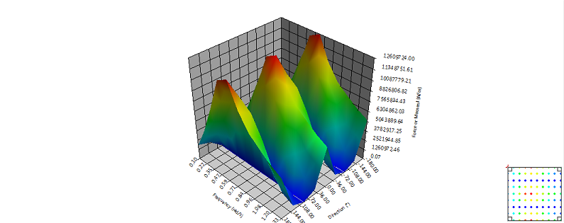
Surface graph presentation: Force/Moment plotted against Direction + Frequency
The Frequency Scale can be modified to be Period Scale if required.
Line Graph Input:
Use the Component input to select which force component to plot, either X, Y, Z for forces or RX, RY, RZ for moments.
When the selected Part includes active Moonpools, the Component is enhanced with additional degrees of freedom in the form of a list of Moonpool pressure modes associated with each active Moonpool under the selected Part. See the note on pressure modes modification and impact on results' validity under Pressure Modes.
When the plot is performed against Direction, then the required frequency can be chosen using the Frequency input.
When the plot is performed against Frequency, then the required direction can be chosen using the Direction input.
Line Graph Output:
Maximum Value and Minimum Value of Angle or Force/Moment and the first Frequency or Direction at which they occur (Abscissa Position of Minimum, Abscissa Position of Maximum). These values can be parameterized by selecting the adjacent check box.
Surface Graph Input:
Use the Component input to select which force component to plot, either X, Y, Z for forces or RX, RY, RZ for moments.
Surface Graph Output:
Maximum Value and Minimum Value of Angle or Force/Moment and the Frequency and Direction at which they occur (Abscissa (X) Position of Minimum, Abscissa (X) Position of Maximum and Ordinate (Y) Position of Minimum, Ordinate (Y) Position of Maximum). These values can be parameterized by selecting the adjacent check box.
Result Description:
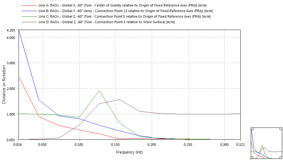
2D or 3D graphs to illustrate how the amplitude and phase of the structure response change with wave direction, frequency or both direction and frequency. You can view RAOs and RAOs taking into account the linearized Morison drag effects, if Linearized Morison Drag is specified.
Plot availability:
Line graph presentation: Phase Angle plotted against either Direction or Frequency
Line graph presentation: Distance/Rotation plotted against either Direction or Frequency
Surface graph presentation: Phase Angle plotted against Direction + Frequency
Surface graph presentation: Distance/Rotation plotted against Direction + Frequency
The Frequency Scale can be modified to be Period Scale if required.
Line Graph Input:
Use the Component input to select which degree of freedom to plot, either X, Y, Z for translation or RX, RY, RZ for rotation.
When the selected Part includes active Moonpools, the Component is enhanced with additional degrees of freedom in the form of a list of Moonpool pressure modes associated to each active Moonpool under the selected Part. See the note on pressure modes modification and impact on results' validity under Pressure Modes.
When the plot is performed against Direction, then the required frequency can be chosen using the Frequency input.
When the plot is performed against Frequency, then the required direction can be chosen using the Direction input.
For a translation RAO, the Reference Point at which the RAO is reported can be the Center of Gravity of the selected Structure, or can be any Connection Point on that structure.
A translation RAO is typically reported for Motion Relative To the Origin of the Fixed Reference Axes (FRA). However, when the Component is set to Global Z and the Reference Point is a Connection Point, the RAO may instead be reported relative to the undiffracted Wave Surface.
Note: For Hydrodynamic Diffraction RAO results, the Connection Point Include in Results option is not required for that Connection Point to be used as a Reference Point.
Line Graph Output:
Maximum Value and Minimum Value of Angle or Distance/Rotation and the first Frequency or Direction at which they occur (Abscissa Position of Minimum, Abscissa Position of Maximum). These values can be parameterized by selecting the adjacent check box.
Surface Graph Input:
Use the Component input to select which degree of freedom to plot, either X, Y, Z for translation or RX, RY, RZ for rotation. For translational degrees of freedom, use the Reference Point and Motion Relative To inputs to set the position and frame of reference for the reported RAOs.
Surface Graph Output:
Maximum Value and Minimum Value of Angle or Distance/Rotation and the Frequency and Direction at which they occur (Abscissa (X) Position of Minimum, Abscissa (X) Position of Maximum and Ordinate (Y) Position of Minimum, Ordinate (Y) Position of Maximum). These values can be parameterized by selecting the adjacent check box.
Result Description:
2D graphs to illustrate how the Radiation Damping or Added Mass varies with frequency.
Plot Availability:
Line Graph Presentation: Radiation Damping or Added Mass plotted against Frequency
The Frequency Scale can be modified to be Period Scale if required.
Line Graph Input:
Use the Subtype and Component inputs to select which value from the Radiation Damping or Added Mass matrix to plot, X, Y, Z for linear components or RX, RY, RZ for rotational components.
When the selected Part includes active Moonpools, the Component and the Subtype are appended with additional degrees of freedom in the form of a list of pressure modes associated to each active Moonpool under the selected Part. See the note on pressure modes modification and impact on results' validity under Pressure Modes.
This image shows how the lists of Subtype and Component have been appended with the Moonpool pressure modes:
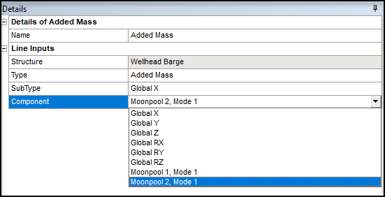
Figure 4.7: Coefficient Locations in Added Mass and Hydrodynamic Damping Matrices details which coefficient is being queried or selected in the Added Mass coefficients matrix for a given structure selection.
The same applies for the radiation damping coefficient matrix.
The combination between the 6 positional degrees of freedom (X,Y,Z, RX, RY, RZ) and the Moonpool pressure modes will result in the following unit system. The SubType and Component selection will give the following type of units:
|
Component► SubType▼ | Translation (X,Y,Z) | Rotational (RX, RY, RZ) | Moonpool Pressure Mode |
| Translation (X,Y,Z) | Tran-Tran | Rot-Tran | Tran-Tran |
| Rotational (RX, RY, RZ) | Tran-Rot | Rot-Rot | Tran-Rot |
| Moonpool Pressure Mode | Tran-Tran | Rot-Tran | Tran-Tran |
Line Graph Output:
Maximum Value and Minimum Value of Radiation Damping and the first Frequency at which they occur (Abscissa Position of Minimum, Abscissa Position of Maximum). These values can be parameterized by selecting the adjacent check box.
Result Description:
2D or 3D graphs to illustrate the mean drift forces/moments applied on the structure and how they change with direction, frequency, or both direction and frequency.
Plot availability:
Line graph presentation: Force/Moment plotted against either Direction or Frequency
Surface graph presentation: Force/Moment plotted against Direction + Frequency
The Frequency Scale can be modified to be Period Scale if required.
Line Graph Input:
Use the Component input to select which force component to plot, either X, Y, or Z for forces or RX, RY, or RZ for moments.
When the plot is performed against Direction, then the required frequency can be chosen using the Frequency input.
When the plot is performed against frequency, then the required direction can be chosen using the Direction input.
Line Graph Output:
Maximum Value and Minimum Value of Angle or Force/Moment and the first Frequency or Direction at which they occur (Abscissa Position of Minimum, Abscissa Position of Maximum). These values can be parameterized by selecting the adjacent check box.
Surface Graph Input:
Use the Component input to select which force component to plot, either X, Y, or Z for forces or RX, RY, or RZ for moments.
Surface Graph Output:
Maximum Value and Minimum Value of Angle or Force/Moment and the Frequency and Direction at which they occur (Abscissa (X) Position of Minimum, Abscissa (X) Position of Maximum and Ordinate (Y) Position of Minimum, Ordinate (Y) Position of Maximum). These values can be parameterized by selecting the adjacent check box.
Result Description:
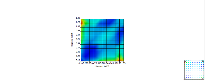
3D graphs to illustrate how these quadratic transfer function (QTF) matrix (which is a force or moment) results change with frequency, for a given direction.
Plot availability:
Surface graph presentation: Phase Angle plotted against Frequency + Frequency
Surface graph presentation: Force/Moment plotted against Frequency + Frequency
The Frequency Scale can be modified to be Period Scale if required.
Surface Graph Input:
Use the Component input to select which force component to plot, either X, Y, Z for forces or RX, RY, RZ for moments.
The required Direction can be chosen.
When Force/Moment plots are performed, the SubType field is shown to enable the selection of the full component, or just the or components.
Surface Graph Output:
Maximum Value and Minimum Value of Angle or Force/Moment and the Frequency and Direction at which they occur (Abscissa (X) Position of Minimum, Abscissa (X) Position of Maximum and Ordinate (Y) Position of Minimum, Ordinate (Y) Position of Maximum). These values can be parameterized by selecting the adjacent check box.
Result Description:
2D or 3D graphs to illustrate how the Splitting Forces (RAO) vary with frequency, direction, or both frequency and direction.
Splitting Forces (RAO) calculations depend upon the masses being accurately defined in the geometry section and are only available for structures that are not included in an Interacting Structure Group.
Note: Splitting Forces (RAO) results are not available for structures containing only a single mass (from Point Mass or Line Body definitions).
Plot availability:
Line graph presentation: Force/Moment vs. Frequency or Direction
Line graph presentation: Phase Angle vs. Frequency or Direction
Surface graph presentation: Force/Moment vs. Frequency + Direction
Surface graph presentation: Phase Angle vs. Frequency + Direction
The Frequency Scale can be modified to be Period Scale if required.
Line Graph Input:
Use the Component input to select which force component to plot, either X, Y, or Z for forces or RX, RY, or RZ for moments.
When the plot is performed against Direction, then the required frequency can be chosen using the Frequency input.
When the plot is performed against Frequency, then the required direction can be chosen using the Direction input.
When Force/Moment plots are performed, the SubType field is shown to enable the selection of the full component, or just the or components.
When Force/Moment plots are performed, use Bounding Box Min Coordinate [X Y Z] to enter the coordinates of one corner of a bounding box and Bounding Box Max Coordinate [X Y Z] to enter the coordinates of the opposite corner of the box. Then enter a Calculation Coordinate [X Y Z] to enter the coordinates of the point about which the moments are calculated. Values entered should be separated by spaces.
Line Graph Output:
Maximum Value and Minimum Value of Angle or Force/Moment and the first Frequency or Direction at which they occur (Abscissa Position of Minimum, Abscissa Position of Maximum). These values can be parameterized by selecting the adjacent check box.
Surface Graph Input:
Use the Component input to select which force component to plot, either X, Y, Z for Forces or RX, RY, RZ for moments.
When Force/Moment plots are performed, the SubType field is shown to enable the selection of the full component, or just the or components.
When Force/Moment plots are performed, use Bounding Box Min Coordinate [X Y Z] to enter the coordinates of one corner of a bounding box and Bounding Box Max Coordinate [X Y Z] to enter the coordinates of the opposite corner of the box. Then enter a Calculation Coordinate [X Y Z] to enter the coordinates of the point about which the moments are calculated. Values entered should be separated by spaces.
Surface Graph Output:
Maximum Value and Minimum Value of Angle or Force/Moment and the Frequency and Direction at which they occur (Abscissa (X) Position of Minimum, Abscissa (X) Position of Maximum and Ordinate (Y) Position of Minimum, Ordinate (Y) Position of Maximum). These values can be parameterized by selecting the adjacent check box.
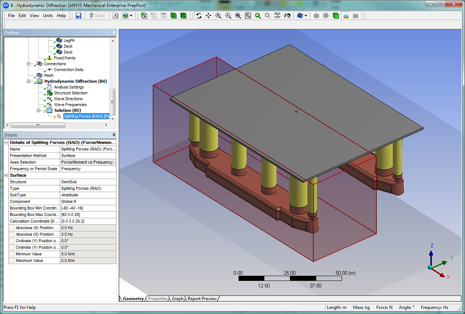
When defining the Bounding Box Min, Max Coordinates [X Y Z], and Calculation Coordinate [X Y Z] for the Splitting Forces (RAO) calculation, while the result object is not yet evaluated, graphical representations of the bounding box and calculation position are shown in the Geometry tab.
Static Bending Moments and Shear Forces can be calculated by the SF/BM (Static) result, and are always plotted along the neutral axis of the vessel. Alternatively, response amplitude operator (RAO) based results can be determined for each wave direction, frequency, and position along the neutral axis. Depending upon the combination of requirements, these will be shown on both 2D and 3D graphs appropriately. When graphs are plotted against Position, the Frequency or Direction can be explicitly selected or they can be enveloped so that the critical result can be identified easily. When graphs are not plotted against Position, then the calculation Position can be specified, and if appropriate, the Frequency or Direction can be explicitly defined (in this situation they cannot be enveloped).
Bending Moment and Shear Force calculations depend upon the masses being accurately defined in the geometry section and will only be permitted if there is only a single structure in the analysis.
Note: If you define only a single Point Mass on a structure, and then request Bending Moment and Shear Force results, the mass is assumed to be distributed over the length of the Part in the selected Neutral Axis direction.
If you define multiple Point Masses, or a Distributed Mass, the mass definitions are split into a number of sections such that the masses are evenly distributed along the length of the Part in the selected Neutral Axis direction (while maintaining the overall CoG position of the Part). Masses from Line Bodies are distributed over the extents of each Line Body, and are then superimposed on the mass distribution.
Result Description:
2D or 3D graphs to illustrate the shear forces/bending moments applied on the structure and how they change with direction, frequency, position along the neutral axis, or combinations of direction/frequency/position.
Plot availability:
Line graph presentation (static): Force/Moment plotted against Position
Line graph presentation (RAO): Force/Moment plotted against either Position, Direction, or Frequency
Line graph presentation (RAO): Phase Angle plotted against either Position, Direction, or Frequency
Surface graph presentation (RAO): Force/Moment plotted against Direction + Frequency, Direction + Position, or Frequency + Position
Surface graph presentation (RAO): Phase Angle plotted against Direction + Frequency, Direction + Position, or Frequency + Position
The Frequency Scale can be modified to be Period Scale if required.
Line Graph Input:
Use the Component input to select which force component to plot, either X, Y, or Z for forces or RX, RY, or RZ for moments.
When the plot is performed against Direction (RAO), then the required frequency can be chosen using the Frequency input and the Position can be entered.
When the plot is performed against Frequency (RAO), then the required direction can be chosen using the Direction input, and the Position can be entered.
When the plot is performed against Position (RAO), then the required direction can be chosen using the Direction input, and the required frequency can be chosen using the Frequency input.
Line Graph Output:
Maximum Value and Minimum Value of Angle or Force/Moment and the first Frequency, Direction, or Position at which they occur (Abscissa Position of Minimum, Abscissa Position of Maximum). These values can be parameterized by selecting the adjacent check box.
Surface Graph Input:
Use the Component input to select which force component to plot, either X, Y, or Z for forces or RX, RY, or RZ for moments.
Surface Graph Output:
Maximum Value and Minimum Value of Angle or Force/Moment and the Frequency and Direction or Frequency and Position or Position and Direction at which they occur (Abscissa (X) Position of Minimum, Abscissa (X) Position of Maximum and Ordinate (Y) Position of Minimum, Ordinate (Y) Position of Maximum). These values can be parameterized by selecting the adjacent check box.
Under the Solution object of a Hydrodynamic Response system, a number of graphs will be available to track the behavior of a number of parameters over time. The graphs are all line graphs, and the following categories of graphs are available:
- 5.11.2.2.1. Wave Surface Elevation
- 5.11.2.2.2. Structure Position
- 5.11.2.2.3. Structure Velocity
- 5.11.2.2.4. Structure Acceleration
- 5.11.2.2.5. Structure Forces
- 5.11.2.2.6. Fender Forces
- 5.11.2.2.7. Fender Motions
- 5.11.2.2.8. Joint Forces
- 5.11.2.2.9. Cable Forces
- 5.11.2.2.10. Tether/Riser Motions
- 5.11.2.2.11. Tether/Riser Tensions
- 5.11.2.2.12. Tether/Riser Shear Force/Bending Moment
- 5.11.2.2.13. Tether/Riser Stresses
- 5.11.2.2.14. Time Step Error
Note: For Time Response results, the table of data points is hidden by default. Use the Show Tabulated Results Data option to show the data points in tabular form.
2D graph to illustrate the elevation of the wave surface over time at a selected position.
Plot Availability:
Line graph presentation: Distance plotted against Time
Line Graph Input:
Use the Reference Point input to select the position at which the Wave Surface Elevation is reported. This may either be at the fixed position specified in the Time Response Analysis Settings or at the (moving) position of any Connection Point that has its Include in Results option to set to yes before the analysis is solved.
Line Graph Output:
Maximum Value and Minimum Value of Wave Surface Elevation and the Time at which they occur (Abscissa Position of Minimum, Abscissa Position of Maximum). These values can be parameterized by clicking the adjacent check box.
Result Description:
2D graphs to illustrate the following response subtypes of the Structure Position during the analysis:
Actual Response
Low Frequency – The low frequency subtype values are obtained by filtering the actual response with a filter which has a cut-off frequency of one third of the frequency of the (10% + 1)th spectral line; that is, with N spectral lines, n = 0.1N + 1, ωcutoff = ωn/3
Wave Frequency – the wave frequency response is that which remains when the low frequency response is subtracted from the actual response
RAO Based – The RAO based motions are those that are calculated using only the RAOs, ignoring the effects of connections (unless these are included as additional matrices in the diffraction analysis), using the applied wave
These values are available in all translational and rotational component directions, and are calculated at the center of gravity or (translation components only) at a Connection Point on the selected structure.
Plot availability:
Line graph presentation: Distance/Rotation plotted against Time
Line Graph Input:
Use the Component input to select which Position component to plot: distance from a defined reference point, X, Y, or Z for translation or RX, RY, or RZ for rotation.
For a translation, the Reference Point at which the result is reported can be the Center of Gravity of the selected Structure, or can be any Connection Point on that structure.
The Motion Relative To input can be used to set the frame of reference for the reported translation. This may be either the Origin of the Fixed Reference Axes (FRA), the Center of Gravity of another structure, a Connection Point on another structure, or a Fixed Point. When the Component is set to Global Z and the Reference Point is a Connection Point, the result may also be reported relative to the Wave Surface. For the latter, the selected Connection Point must have its Include in Results option set to Yes before the analysis is solved, and the result SubType must be set to Actual Response.
Line Graph Output:
Maximum Value and Minimum Value of Structure Position and the Time at which they occur (Abscissa Position of Minimum, Abscissa Position of Maximum). These values can be parameterized by selecting the adjacent check box.
Result Description:
2D graphs to illustrate the following response subtypes of the Structure Velocity during the analysis:
Actual Response
Low Frequency – The low frequency subtype values are obtained by filtering the actual response with a filter which has a cut-off frequency of one third of the frequency of the (10% + 1)th spectral line; that is, with N spectral lines, n = 0.1N + 1, ωcutoff = ωn/3
Wave Frequency – the wave frequency response is that which remains when the low frequency response is subtracted from the actual response
RAO Based – The RAO based motions are those that are calculated using only the RAOs, ignoring the effects of connections (unless these are included as additional matrices in the diffraction analysis), using the applied wave
These values are available in all translational and rotational component directions, and are calculated at the center of gravity or (translation components only) at a Connection Point on the selected structure.
Plot availability:
Line graph presentation: Velocity plotted against Time
Line Graph Input:
Use the Component input to select which Velocity component to plot, either X, Y, or Z for translational velocity or RX, RY, or RZ for rotational velocity.
For a translational velocity, the Reference Point at which the result is reported can be the Center of Gravity of the selected Structure, or can be any Connection Point on that structure.
The Motion Relative To input can be used to set the frame of reference for the reported translational velocity. This may be either the Origin of the Fixed Reference Axes (FRA), the Center of Gravity of another structure, or a Connection Point on another structure. When the Component is set to Global Z and the Reference Point is a Connection Point, the result may also be reported relative to the Wave Surface. For the latter, the selected Connection Point must have its Include in Results option set to Yes before the analysis is solved, and the result SubType must be set to Actual Response.
Line Graph Output:
Maximum Value and Minimum Value of Structure Velocity and the Time at which they occur (Abscissa Position of Minimum, Abscissa Position of Maximum). These values can be parameterized by selecting the adjacent check box.
Result Description:
2D graphs to illustrate the following response subtypes of the Structure Acceleration during the analysis:
Actual Response
Low Frequency – The low frequency subtype values are obtained by filtering the actual response with a filter which has a cut-off frequency of one third of the frequency of the (10% + 1)th spectral line; that is, with N spectral lines, n = 0.1N + 1, ωcutoff = ωn/3
Wave Frequency – the wave frequency response is that which remains when the low frequency response is subtracted from the actual response
RAO Based – The RAO based motions are those that are calculated using only the RAOs, ignoring the effects of connections (unless these are included as additional matrices in the diffraction analysis), using the applied wave
These values are available in all translational and rotational component directions, and are calculated at the center of gravity or (translation components only) at a Connection Point on the selected structure.
Plot availability:
Line graph presentation: Acceleration plotted against Time
Line Graph Input:
Use the Component input to select which Acceleration component to plot, either X, Y, or Z for translational acceleration or RX, RY, or RZ for rotational acceleration.
For a translational acceleration, the Reference Point at which the result is reported can be the Center of Gravity of the selected Structure, or can be any Connection Point on that structure.
The Motion Relative To input can be used to set the frame of reference for the reported translational acceleration. This may be either the Origin of the Fixed Reference Axes (FRA), the Center of Gravity of another structure, or a Connection Point on another structure. When the Component is set to Global Z and the Reference Point is a Connection Point, the result may also be reported relative to the Wave Surface. For the latter, the selected Connection Point must have its Include in Results option set to Yes before the analysis is solved, and the result SubType must be set to Actual Response.
Line Graph Output:
Maximum Value and Minimum Value of Structure Acceleration and the Time at which they occur (Abscissa Position of Minimum, Abscissa Position of Maximum). These values can be parameterized by selecting the adjacent check box.
Result Description:
2D graphs to illustrate the following response subtypes of the Structure Forces during the analysis:
Total Force/Moment
Mooring Sum Only
Gyroscopic Only
Diffraction Only
Linear Damping Only
Morison Drag Only
Drift Only
Froude-Krylov Only
Gravitation Only
Current Drag Only
Wave Inertia Only
Hydrostatic Only
Wind Only
Slam Only
Point Only
Yaw Drag Only
Slender Body Only
Radiation Only
Fluid Momentum Only
Fluid Gyroscopic Only
Externally Applied Only
Linear Wave Drift Damping Only
Maneuvering Force Only
The sum of forces for each individual subtype will be shown in the graph. If all of the forces are taken in combination, they will form the result available by the Total Force/Moment subtype. In the case where the force is not included in the analysis the subtype will not be available for selection.
Note: When including drift effects, the Froude-Krylov Only excludes those calculated on diffracting panels; instead, these are included under the Diffraction Forces.
These values are calculated at the center of gravity and are available in all translational and rotational component directions.
Plot availability:
Line graph presentation: Force/Moment plotted against Time
Line Graph Input:
Use the Component input to select which Structure Force/Moment component to plot, either X, Y, or Z for force components or RX, RY, or RZ for rotational components.
Line Graph Output:
Maximum Value and Minimum Value of the Structure Force and the Time at which they occur (Abscissa Position of Minimum, Abscissa Position of Maximum). These values can be parameterized by selecting the adjacent check box.
Result Description:
2D graphs to illustrate the fender forces during the analysis. You must select the Structure and Connection to that structure (connected Fender) for which you want to display the results.
Plot availability:
Line graph presentation: Force plotted against Time
Line Graph Input:
Use the Component input to select which Fender Force component to plot; either X, Y, or Z force components, or one of the following: Total Force, Elastic Force, Damping Force, or Friction Force.
Line Graph Output:
Maximum Value and Minimum Value of the Fender Force and the Time at which they occur (Abscissa Position of Minimum, Abscissa Position of Maximum). These values can be parameterized by selecting the adjacent check box.
Result Description:
2D graphs to illustrate the fender motions during the analysis. You must select the Structure and Connection to that structure (connected Fender) for which you want to display the results.
Plot Availability:
Line graph presentation: Distance plotted against Time
Line Graph Input:
Use the Component input to select which Fender Motion to plot; either Compression, Horizontal Movement, or Upward (Z) Movement.
Line Graph Output:
Maximum Value and Minimum Value of the Fender Motion and the Time at which they occur (Abscissa Position of Minimum, Abscissa Position of Maximum). These values can be parameterized by selecting the adjacent check box.
Result Description:
2D graphs to illustrate the joint forces during the analysis. You must select the Structure and Connection to that structure (connected Joint) for which you want to display the results.
Plot availability:
Line graph presentation: Force/Moment plotted against Time
Line Graph Input:
Use the Component input to select which Joint Force component to plot; either X, Y, or Z force components, or RX, RY, or RZ rotational components.
Line Graph Output:
Maximum Value and Minimum Value of the Joint Force and the Time at which they occur (Abscissa Position of Minimum, Abscissa Position of Maximum). These values can be parameterized by selecting the adjacent check box.
The force components are available for each cable. For multi-segment catenary cables, section tension is also available.
Result Description:
2D graphs to illustrate cable tension during the analysis.
Whole Cable Forces
Cable Section Tension
Plot availability:
Line graph presentation: Force or Tension plotted against Time
Line Graph Input:
For Whole Cable Forces, use the Connection field to select which cable's characteristics to plot. Use the Component input to select which Cable Force component to plot; either X, Y, or Z force components, or Anchor Uplift, Tension, or Laid Length.
For Cable Section Tension, use the Connection field to select which catenary cable's characteristics to plot. Use the Cable Section field to select the Catenary Section for which you want to plot section tension.
Line Graph Output:
Maximum Value and Minimum Value of Cable Force/Tension and the Time at which they occur (Abscissa Position of Minimum, Abscissa Position of Maximum). These values can be parameterized by selecting the adjacent check box.
Result Description:
2D graphs to illustrate the variation in the following results of a tether/riser node during the analysis:
Displacement
Velocity
Acceleration
You must select the Structure and Connection to that structure (connected tether/riser) for which you want to display the results.
Tether/Riser motion results are output in the Tether/Riser Local Axes (TLA), which are described in Tethers/Risers. As the TLA points from the Start Fixed Point to the End Connection Point of the Tether/Riser, where the End Connection Point will be moving with its associated Structure, the motions of the first and last nodes will always be zero.
Plot Availability:
Line graph presentation: Result plotted against Time
Line Graph Input:
Use the Tether/Riser Node input to select the node for which results will be displayed. Use the Component input to select which tether/riser nodal result component to plot: either X or Y translational components, or RX or RY rotational components.
Line Graph Output:
Maximum Value and Minimum Value of the tether/riser nodal result and the times at which they occur (Abscissa Position of Minimum, Abscissa Position of Maximum). These values can be parameterized by selecting the adjacent check box.
Result Description:
2D graphs to illustrate the following subtypes of the Tether/Riser Tensions during the analysis:
Connection Point Tension
Section Tension
Nodal Tension
Wall Tension
You must select the Structure and Connection to that structure (connected tether/riser) for which you want to display the results.
Plot availability:
Line graph presentation: Force plotted against Time
Line Graph Input:
The input required depends on the selected graph subtype.
For Connection Point Tension, no other input in required; the graph will display the Tether/Riser tensions at the structure Connection Point.
For Section Tension, use the Tether Section input to select the section for which results will be displayed.
For Nodal Tension, use the Tether/Riser Node input to select the node for which results will be displayed. The definition elevation of the selected node is shown for reference.
For Wall Tension, use the Tether/Riser Element input to select an element along the tether, and the Tether/Riser Element End input to select the end of that element for which results will be displayed. The definition elevation of the selected element end is shown for reference.
Line Graph Output:
Maximum Value and Minimum Value of tether/riser tensions and the times at which they occur (Abscissa Position of Minimum, Abscissa Position of Maximum). These values can be parameterized by selecting the adjacent check box.
Result Description:
2D graphs to illustrate the following subtypes of the Tether/Riser Shear Force/Bending Moment during the analysis:
Element Shear Force/Bending Moment
Connection Point Shear Force/Bending Moment
You must select the Structure and Connection to that structure (connected tether/riser) for which you want to display the results.
Plot availability:
Line graph presentation: Force/Moment plotted against Time
Line Graph Input:
If the selected graph subtype is Element Shear Force/Bending Moment, use the Tether/Riser Element input to select an element along the tether, and the Tether/Riser Element End input to select the end of that element for which results will be displayed. The definition elevation of the selected element end is shown for reference.
Regardless of the selected graph subtype, you should use the Component input to select which Shear Force/Bending Moment component to plot: Local Tether/Riser X or Y for shear force components, or Local Tether/Riser RX or RY for bending moment components.
Line Graph Output:
Maximum Value and Minimum Value of tether/riser shear forces/bending moments and the times at which they occur (Abscissa Position of Minimum, Abscissa Position of Maximum). These values can be parameterized by selecting the adjacent check box.
Result Description:
2D graphs to illustrate the following subtypes of the Tether/Riser Stresses during the analysis:
Shear Stress
Maximum Bending + Axial Stress
Minimum Bending + Axial Stress
Von Mises Stress
Y Bending Stress
You must select the Structure and Connection to that structure (connected tether/riser) for which you want to display the results.
Plot availability:
Line graph presentation: Stress plotted against Time
Line Graph Input:
Use the Tether/Riser Element input to select an element along the tether, and the Tether/Riser Element End input to select the end of that element for which results will be displayed. The definition elevation of the selected element end is shown for reference.
Line Graph Output:
Maximum Value and Minimum Value of tether/riser stresses and the times at which they occur (Abscissa Position of Minimum, Abscissa Position of Maximum). These values can be parameterized by selecting the adjacent check box.
The movement error is graphed for each time step. The program outputs the movement error at each time step in each degree of freedom which is related to the chosen time step. These errors can always be reduced by shortening the time step.
Result Description:
2D graphs to illustrate the movement error per step during the analysis.
Plot availability:
Line graph presentation: Movement Error plotted against Time
Line Graph Input:
None.
Line Graph Output:
Maximum Value and Minimum Value of Movement Error and the Time at which they occur (Abscissa Position of Minimum, Abscissa Position of Maximum). These values can be parameterized by selecting the adjacent check box.
A number of line graphs may be added under the Solution object of a Frequency Domain Analysis system to illustrate the variation of different parameters with frequency. The following topics are available:
Result Description:
2-D graphs to illustrate an input wave energy spectrum, over the range of frequencies assumed or defined in an active Irregular Wave object, from the present analysis. Note that a Wave Spectrum may be plotted on the same axes as a Structure Position Response Spectrum by changing the plot Type of an additional Line to Position Response Spectra.
Plot Availability:
Line graph presentation: Spectral Density plotted against Frequency
The Frequency Scale can be modified to be Period Scale if required.
Line Graph Input:
Use the Wave Spectrum Input to select an Irregular Wave spectrum to plot.
If the selected Irregular Wave contains more than one sub-spectrum and/or Cross Swell Spectrum, the Spectrum Sub-Direction input should be used to select a specific sub-spectrum for plotting.
Line Graph Output:
Maximum Value and Minimum Value of Spectral Density, and the Frequencies at which these occur (Abscissa Position of Minimum, Abscissa Position of Maximum). These values can be parameterized by selecting the adjacent check box.
Result Description:
2-D graphs to illustrate various structural force and motion responses over the range of frequencies used in the present Frequency Statistical Analysis. The direction used for output of Motion RAOs and Transfer Functions is that specified in Spectrum Sub-Direction of Output for RAOs under Analysis Settings. Note that a Position Response Spectrum may be plotted on the same axes as a Wave Spectrum by changing the plot Type of an additional Line to Wave Spectra, and a Force/Moment Response Spectrum may be plotted on the same axes as a Joint Reaction Spectrum by changing the plot Type of an additional Line to Joint Reaction Spectra.
Plot Availability:
Line graph presentation: Response Amplitude Operator (RAO) plotted against Frequency
Line graph presentation: Force/Moment Response Spectrum plotted against Frequency
Line graph presentation: Position Response Spectrum plotted against Frequency
Line graph presentation: Velocity Response Spectrum plotted against Frequency
Line graph presentation: Acceleration Response Spectrum plotted against Frequency
Line graph presentation: Transfer Function plotted against Frequency
The Frequency Scale can be modified to be Period Scale if required.
Line Graph Input:
Use the Structure input to select a structure from the present analysis.
Use the Component input to select which component to plot: either X, Y, Z for forces/translations or RX, RY, RZ for moments/rotations.
For translational Motion RAOs and translational Position/Velocity/Acceleration Response Spectra, the Reference Point at which the result is reported can be the Center of Gravity of the selected Structure, or can be any Connection Point on that structure. For the latter, the selected Connection Point must have it Include in Results option set to Yes before the analysis is solved.
Translational Motion RAOs and translational Position/Velocity/Acceleration Response Spectra are typically reported for Motion Relative To the Origin of the Fixed Reference Axes (FRA). However, when the Component is set to Global Z and the Reference Point is a Connection Point, the translational RAO/Response Spectrum may instead be be reported relative to the Wave Surface. Alternatively, if the Reference Point is a Connection Point and the Axis System for Significant Motions and Nodal Response option under Analysis Settings is set to Local Structure Axes, Motion Relative To can be set to the Origin of the Local Structure Axes (LSA).
Line Graph Output:
Maximum Value and Minimum Value of the selected Structure Response variable, and the Frequencies at which these occur (Abscissa Position of Minimum, Abscissa Position of Maximum). These values can be parameterized by selected the adjacent check box.
Result Description:
2-D graphs to illustrate forces and reactions in cables, fenders, and joints over the range of frequencies used in the present Frequency Statistical Analysis. The direction used for output of Cable Tension RAOs and Fender Force RAOs is that specified in Spectrum Sub-Direction of Output for RAOs under Analysis Settings.
Plot Availability:
Line graph presentation: Cable Tension Response Amplitude Operator (RAO) plotted against Frequency
Line graph presentation: Fender Force Response Amplitude Operator (RAO) plotted against Frequency
Line graph presentation: Joint Reaction Spectrum plotted against Frequency
The Frequency Scale can be modified to be Period Scale if required.
Line Graph Input:
Use the Structure input to select a structure from the present analysis.
Use the Connection input to select a valid connection for that structure.
For Joint Reaction Spectra, use the Component input to select which component to plot: either X, Y, Z for forces, or RX, RY, RZ for moments.
Line Graph Output:
Maximum Value and Minimum Value of the selected Connection Response variable, and the Frequencies at which these occur (Abscissa Position of Minimum, Abscissa Position of Maximum). These values can be parameterized by selecting the adjacent check box.
Under the Solution object of a Stability Response analysis, a number of graphs will be available to track the behavior of a number of parameters as they vary with each iteration step. The graphs are all line graphs, and the following categories are available:
Result Description:
2D graphs to illustrate the Structure Position during the analysis.
These values are available in all translational and rotational component directions, and are calculated at the center of gravity or (translation components only) at a Connection Point on the selected structure.
Plot availability:
Line graph presentation: Distance/Rotation plotted against Iteration Step
Line Graph Input:
Use the Component input to select which Position component to plot, either X, Y, or Z for translation or RX, RY, or RZ for rotation.
For a translation, the Reference Point at which the result is reported can be the Center of Gravity of the selected Structure, or can be any Connection Point on that structure.
The Motion Relative To input can be used to set the frame of reference for the reported translation. This may be either the Origin of the Fixed Reference Axes (FRA), the Center of Gravity of another structure, a Connection Point on another structure, or a Fixed Point.
Note: For Hydrodynamic Equilibrium Results, the Connection Point Include in Results option is not required for that Connection Point to be used as a Reference Point.
Line Graph Output:
Initial Value and Final Value of Structure Position. These values can be parameterized by selecting the adjacent check box.
Result Description:
2D graphs to illustrate the following response subtypes of the Structure Forces during the analysis:
All
Mooring Sum Only
Articulation Sum Only
Morison Drag Only
Drift Only
Gravitational Only
Current Drag Only
Hydrostatic Only
Wind Only
Point Only
Slender Body Only
Externally Applied Only
The sum of forces for each individual subtype will be shown in the graph. If all of the forces are taken in combination, they will form the result available by the All subtype. In the case where the force is not included in the analysis (e.g. Drift Forces, when drift is excluded) the subtype will produce zero values.
Note: When including drift effects, the Froude-Krylov Only excludes those calculated on diffracting panels; instead, these are included under the Diffraction Forces.
These values are calculated at the center of gravity and are available in all translational and rotational component directions.
Plot availability:
Line graph presentation: Force/Moment plotted against Iteration Step
Line Graph Input:
Use the Component input to select which Structure Force/Moment component to plot, either X, Y, or Z for force components or RX, RY, or RZ for rotational components.
Line Graph Output:
Initial Value and Final Value of the Structure Force. These values can be parameterized by selecting the adjacent check box.
Result Description:
2D graphs to illustrate the fender forces during the analysis. You must select the Structure and Connection to that structure (connected Fender) for which you want to display the results.
Plot availability:
Line graph presentation: Force plotted against Iteration Step
Line Graph Input:
Use the Component input to select which Fender Force component to plot; either X, Y, or Z force components, or one of the following: Total Force, Elastic Force, Damping Force, or Friction Force.
Line Graph Output:
Initial Value and Final Value of the Fender Force. These values can be parameterized by selecting the adjacent check box.
Result Description:
2D graphs to illustrate the fender motions during the analysis. You must select the Structure and Connection to that structure (connected Fender) for which you want to display the results.
Plot Availability:
Line graph presentation: Distance plotted against Iteration Step
Line Graph Input:
Use the Component input to select which Fender Force component to plot; either Compression, Horizontal Movement, or Upward (Z) Movement.
Line Graph Output:
Initial Value and Final Value of the Fender Motion. These values can be parameterized by selecting the adjacent check box.
Result Description:
2D graphs to illustrate the joint forces during the analysis. You must select the Structure and Connection to that structure (connected Joint) for which you want to display the results.
Plot availability:
Line graph presentation: Force/Moment plotted against Iteration Step
Line Graph Input:
Use the Component input to select which Joint Force component to plot; either X, Y, or Z force components, or RX, RY, or RZ rotational components.
Line Graph Output:
Initial Value and Final Value of the Joint Force. These values can be parameterized by selecting the adjacent check box.
The force components are available for each cable. For catenary cables sections, section tension is also available.
Result Description:
2D graphs to illustrate cable tension during the analysis.
Whole Cable Forces
Cable Section Tension
Plot availability:
Line graph presentation: Force or Tension plotted against Iteration Step
Line Graph Input:
For Whole Cable Forces, use the Connection field to select which cable's characteristics to plot. Use the Component input to select which Cable Force component to plot; either X, Y, or Z force components, or Anchor Uplift, Tension, or Laid Length.
For Cable Section Tension, use the Connection field to select which catenary cable's characteristics to plot. Use the Cable Section field to select the Catenary Section for which you want to plot section tension.
Line Graph Output:
Initial Value and Final Value of Cable Force/Tension. These values can be parameterized by selecting the adjacent check box.
Result Description:
2D graphs to illustrate the following subtypes of the Tether/Riser Tensions during the analysis:
Connection Point Tension
Section Tension
You must select the Structure and Connection to that structure (connected tether/riser) for which you want to display the results.
Plot availability:
Line graph presentation: Force plotted against Iteration Step
Line Graph Input:
The input required depends on the selected graph subtype.
For Connection Point Tension, no other input in required; the graph will display the Tether/Riser tensions at the structure Connection Point.
For Section Tension, use the Tether Section input to select the section for which results will be displayed.
Line Graph Output:
Initial Value and Final Value of Tether/Riser tensions. These values can be parameterized by selecting the adjacent check box.
Result Description:
2D graphs to illustrate the Tether/Riser Shear Force/Bending Moment at the structure Connection Point during the analysis.
You must select the Structure and Connection to that structure (connected tether/riser) for which you want to display the results.
Plot availability:
Line graph presentation: Force/Moment plotted against Iteration Step
Line Graph Input:
Use the Component input to select which Connection Point Shear Force/Bending Moment component to plot: Local Tether/Riser X or Y for shear force components, or Local Tether/Riser RX or RY for bending moment components.
Line Graph Output:
Initial Value and Final Value of Tether/Riser shear forces/bending moments. These values can be parameterized by selecting the adjacent check box.
The ratio of movement at each iterative step to the maximum allowable error is graphed for each iteration step. These errors can always be reduced by decreasing the Movement Limitation or increasing the Maximum Error in Equilibrium Position.
Result Description:
2D graphs to illustrate the relative error per step during the analysis.
Plot availability:
Line graph presentation: Relative Error plotted against Iteration Step
Line Graph Input:
None.
Line Graph Output:
Initial Value and Final Value of Relative Error. These values can be parameterized by selecting the adjacent check box.