The hybrid integration rule is recommended for transient nonisothermal flow or heat conduction problems involving thermal shocks (for example, a glass pressing problem). Indeed, in cases that involve thermal shocks, this technique has been found to remove the numerical wiggles of the temperature field. The hybrid integration rule is computationally slightly more expensive than the standard one, while there is no extra cost regarding memory. If no thermal shock is present, the standard and hybrid integration rules provide essentially the same results.

In order to select the hybrid integration rule, you need to perform the following steps:

The hybrid method is only available for the following:

For 2D (and 2D 1/2) flows, the default method involves a quadratic representation of the velocity field and a linear-continuous representation of the pressure field. Such a representation is valid for quadrilateral and triangular elements, and has been used extensively in fluid mechanics problems.

In the Interpolation menu in Ansys Polydata, this option corresponds to the Quadratic velocities, linear pressure menu item, which is enabled by default.

The quadratic-linear representation, however, is characterized by a relatively low number of incompressibility constraints in comparison with the momentum equations. A more accurate method can be obtained with a discontinuous representation for the pressure, which then becomes a first-order polynomial in each element. This quadratic-linear-discontinuous representation is sometimes used in free surface or thermal convection problems. In the Interpolation menu in Ansys Polydata, this option corresponds to the Quadratic velocities, linear discontinuous pressure menu item.

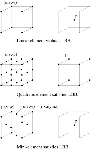
A linear representation of the velocity field with a constant pressure in each element is also available, although this method does not satisfy the Ladyzenskaja-Babuska-Brezzi (LBB) criterion [20] (or min-max condition). To avoid spurious pressure modes, the pressure is stabilized by an artificial compressibility term. The linear representation is a computationally inexpensive method that can give satisfactory results with appropriate boundary conditions (mostly of the Neumann type). In the Interpolation menu in Ansys Polydata, this option corresponds to the Linear velocities, constant pressure menu item.

A linear representation of the velocity field combined with a linear representation of the pressure field in each element is set as the default interpolation for 3D generalized Newtonian flows. While this interpolation is also available for viscoelastic flows, it is, however, not available when the mesh superposition technique is invoked. As this interpolation does not respect the LBB criterion, the linear pressure is stabilized by an artificial compressibility term to avoid spurious pressure modes. In the Interpolation menu in Ansys Polydata, this option corresponds to the Linear velocities, linear pressure menu item.

The Linear velocities, linear pressure representation is less expensive than the Linear velocities, constant pressure option when the mesh contains a large number of tetrahedra. Indeed, in a mesh consisting exclusively of tetrahedra, there are fewer nodes than elements, hence there are fewer pressure unknowns with a linear interpolation. The cost for other meshes is not significantly higher with a slightly better accuracy on pressure in some cases. Indeed, with a constant pressure per element, it is not always possible to get a good representation of the pressure, especially with a coarse mesh.

As mentioned previously, with the Linear velocities, constant pressure option, the linear representation of the velocity violates the LBB criterion, but the stabilization of the incompressibility equation fixes the issue. The linear interpolation of the velocity has a low computational cost (it is the cheapest for a mesh composed of hexahedra) and is one of the only interpolation available for 3D cases involving contact (for example, as encountered in blow molding and thermoforming). In some configurations it also leads to smoother velocity profiles compared to the mini-element representation, which is especially important in nonisothermal cases.

The mini-element representation of the velocity was developed by Fortin [13]. The mini-element is implemented as a correction to the linear element: a degree of freedom is introduced on the midfaces of the elements, but only for the normal part of the velocity vector, as indicated in Figure 10.3: Implementation of the Mini-Element. This minimizes the cost of the correction and solves all problems linked to incompressibility (the LBB condition), it therefore does not require pressure stabilization.

The cost of the mini-element is similar to that of the simpler linear element, but the mini-element scheme is more accurate. It provides reasonably accurate results at lower cost than the quadratic methods. In the Interpolation menu in Ansys Polydata, the mini-element option corresponds to the Mini-element for velocities, constant pressure menu item.

The mini-element uses a piecewise-constant finite-element pressure representation. This can cause problems for some meshes that exhibit a large aspect ratio (that is, meshes for which the dimension in one direction is much smaller than in another direction, so that a strong pressure gradient develops). The problem becomes worse if the mesh includes elements that are strongly deformed (that is, elements whose opposite sides are of different dimensions).

In order to address this problem without imposing the use of the CPU-intensive quadratic approximation (described below), a combination of the mini-element with a linear pressure is provided. In the Interpolation menu in Ansys Polydata, the mini-element with linear pressure option corresponds to the Mini-element for velocities, linear pressure menu item.

Figure 10.3: Implementation of the Mini-Element

This option greatly improves the pressure representation in cases where the accuracy of the standard mini-element is not good. The mini-element with linear pressure uses "bubble" velocity shape functions at element centers. Even with this additional bubble shape function at the element centers, there are rare boundary condition cases where the element violates incompressibility conditions. In order to avoid solution difficulties, the incompressibility equation is stabilized with an artificial compressibility that is small enough to not be a problem in practical flow situations.

The quadratic-linear representation (Quadratic velocities, linear pressure) is the most accurate and the most expensive of all representations, and the quadratic-linear-discontinuous representation (Quadratic velocities, linear discontinuous pressure) may be more accurate for free surface or thermal convection problems. However, using the quadratic representation on a dense 3D finite-element mesh can be computationally expensive and require a significant amount of memory.

For a shear-rate-dependent viscosity, Ansys Polyflow will, by default, use Newton-Raphson iterations to solve the nonlinearities. In the Interpolation menu in Ansys Polydata, this option corresponds to the Newton iterations on viscosity(g) item listed in the Current setup at the top of the menu. (Since it is enabled by default, it will not appear in the menu item list itself, only in the Current setup list.)

For power-law or Bird-Carreau fluids with a power-law index less than 0.7, Picard (fixed-point) iterations are recommended instead of the default Newton-Raphson iterations.

The Picard scheme typically requires 20 iterations or more to converge to a tolerance of 10^-3, while the Newton-Raphson scheme often requires 3 to 4 iterations. However, the radius of the convergence disk for the Newton-Raphson scheme is small for power-law fluids. The Picard scheme provides better convergence behavior when the power-law index is low. In the Interpolation menu in Ansys Polydata, this option corresponds to the Picard iterations on viscosity(g) menu item.

Another option for a low power-law index is to use the default Newton-Raphson technique with an evolution scheme that gradually decreases the power-law index. See Using Evolution to Compute Generalized Newtonian Flow for details.

Another alternative may consist of activating the convergence strategy for rheology and slipping, available in the Numerical parameters menu (see Convergence Strategy for Rheology and Slipping).

For nonisothermal flows, several types of interpolation are available in Ansys Polyflow to calculate the temperature field. You should select the interpolation type according to the Péclet number:

(10–26)

where is a characteristic velocity of the flow, and is a characteristic length of the flow. When the Péclet number is low, you should use quadratic elements (the default) for the temperature in 2D. In the Interpolation menu in Ansys Polydata, this option corresponds to the Quadratic element for temperature menu item.

For low-Péclet-number 3D simulations where you need to reduce the CPU time and/or problem size, you can use linear elements for temperature instead of the default quadratic elements. In the Interpolation menu in Ansys Polydata, this option corresponds to the Linear element for temperature menu item.

For moderate Péclet numbers, subdivision into linear subelements with a Galerkin method is recommended for the energy equation. In the Interpolation menu in Ansys Polydata, this option corresponds to the 2x2 element for temperature menu item.

For flows with high Péclet numbers, you should use subelements with a streamline-upwind Petrov-Galerkin method for the energy equation. In the Interpolation menu in Ansys Polydata, this option corresponds to the 4x4 element for temperature menu item combined with the Upwinding in the energy equation menu item.

This method refines the mesh for temperature without increasing the cost of the velocity-pressure calculation. Note, however, that the 4x4 element for temperature is not available for 3D simulations. For high-Péclet-number 3D cases, the 2x2 element for temperature is recommended instead.

The need for a special treatment of the energy equation can be seen when the temperature field exhibits wiggles (oscillations). These indicate that the mesh is too coarse. Such behavior also occurs in convection-dominated problems.

You can assign different interpolation types to different subdomains, using the Sub-interpolation option in the Interpolation menu. For example, you can use subelements in one subdomain, and in another. See Problem Setup for details.

Linear coordinates (the default) are recommended for flows that do not involve surface tension. Quadratic coordinates should be used for flows involving surface tension (for example, coating flows). See Controlling the Interpolation for more details.