


When solving an extrusion problem it is possible that two free surfaces will come into contact. For the implementation of fluid-fluid contact it is assumed that the two fluids do not slip on each other. This means that the vertices of one fluid in contact with the other fluid will move with the same local velocity, as shown in Figure 15.5: Contact Detection.
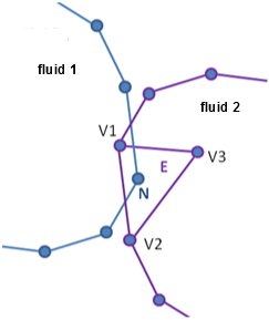
The vertex N of fluid 1 is in the
element E of fluid 2. This element
E is defined by the 3 vertices { }. Vertex N of fluid 1 is
forced to move with fluid 2 by the following constraint:
}. Vertex N of fluid 1 is
forced to move with fluid 2 by the following constraint:
 | (15–22) |
The velocity at vertex N is a linear combination of the
velocities at vertices  ,
,  , and
, and  . The coupling coefficients
  ,
,  , and
, and  are evaluated following the local position of vertex
N in element E.
are evaluated following the local position of vertex
N in element E.
As shown in Figure 15.5: Contact Detection, the creation of the
constraints depends on the detection of contact of one fluid into the other one.
Similar to the contact detection in blow molding there is a numerical parameter for
detecting fluid-fluid contact called element dilatation. A
second parameter, specific to the fluid-fluid contact is the minimum
coupling coefficient. This parameter allows you to neglect some
coefficient— ,
,  or
or  (in Equation 15–22)—if the coefficient's value is lower than that minimum.
An additional field, named fluid-contact, is defined on the union of the two free surfaces. It allows Polyflow to see which vertices are in contact (value of 1), and those that are not (value of 0).
Note: Polyflow automatically creates planes of symmetry when and where they are required during the corrections step of the fluid-fluid contact mapping. If needed, you can modify or deactivate these symmetry planes in the Planes of symmetry management menu (see Mapping for additional information).
This feature is not available for shells or films.